FElupe documentation#
FElupe is a Python 3.8+ 🐍 finite element analysis package 📦 focussing on the formulation and numerical solution of nonlinear problems in continuum mechanics 🔧 of solid bodies 🚂. Its name is a combination of FE (finite element) and the german word Lupe 🔍 (magnifying glass) as a synonym for getting an insight 📖 how a finite element analysis code 🧮 looks like under the hood 🕳️.
Highlights
high-level finite-element-analysis API
flexible building blocks for finite element assembly
hyperelastic
integral (weak) formsstraight-forward definition of
mixed-fields
Installation#
Install Python, fire up 🔥 a terminal and run 🏃

pip install felupe[all]
where [all] is a combination of [io,parallel,plot,progress,view] and installs all optional dependencies. FElupe has minimal requirements, all available at PyPI supporting all platforms.
numpy for array operations
scipy for sparse matrices
tensortrax for automatic differentiation
In order to make use of all features of FElupe 💎💰💍👑💎, it is suggested to install all optional dependencies.
Getting Started#
This minimal code-block covers the essential high-level parts of creating and solving problems with FElupe. As an introductory example 👨🏫, a quarter model of a solid cube with hyperelastic material behaviour is subjected to a uniaxial() elongation applied at a clamped end-face.
First, let’s import FElupe and create a meshed cube out of hexahedron cells with a given number of points per axis. A numeric region, pre-defined for hexahedrons, is created on the mesh. A vector-valued displacement field is initiated on the region. Next, a field container is created on top of this field.
A uniaxial() load case is applied on the displacement field stored inside the field container. This involves setting up symmetry() planes as well as the absolute value of the prescribed displacement at the mesh-points on the right-end face of the cube. The right-end face is clamped 🛠️: only displacements in direction x are allowed. The dict of boundary conditions for this pre-defined load case are returned as boundaries and the partitioned degrees of freedom as well as the external displacements are stored within the returned dict loadcase.
An isotropic pseudo-elastic Ogden-Roxburgh Mullins-softening model formulation in combination with an isotropic hyperelastic Neo-Hookean material formulation is applied on the displacement field of a nearly-incompressible solid body.
A step generates the consecutive substep-movements of a given boundary condition. The step is further added to a list of steps of a job 👩💻 (here, a characteristic curve 📈 job is used). During evaluation ⏳, each substep of each step is solved by an iterative Newton-Rhapson procedure ⚖️. The solution is exported after each completed substep as a time-series ⌚ XDMF file. Finally, the result of the last completed substep is plotted.
Slightly modified code-blocks are provided for different kind of analyses and element formulations.
import felupe as fem

mesh = fem.Cube(n=6)
region = fem.RegionHexahedron(mesh)
field = fem.FieldContainer([fem.Field(region, dim=3)])

boundaries, loadcase = fem.dof.uniaxial(field, clamped=True)

umat = fem.NeoHooke(mu=1)
solid = fem.SolidBodyNearlyIncompressible(umat, field, bulk=5000)

move = fem.math.linsteps([0, 1], num=5)
step = fem.Step(items=[solid], ramp={boundaries["move"]: move}, boundaries=boundaries)

job = fem.CharacteristicCurve(steps=[step], boundary=boundaries["move"])
job.evaluate(filename="result.xdmf")
fig, ax = job.plot(
    xlabel="Displacement $d_1$ in mm $\longrightarrow$",
    ylabel="Normal Force $F_1$ in N $\longrightarrow$",
)
solid.plot(
    "Principal Values of Cauchy Stress"
).show()
import felupe as fem

mesh = fem.Cube(n=(9, 5, 5)).add_midpoints_edges()
region = fem.RegionQuadraticHexahedron(mesh)
field = fem.FieldContainer([fem.Field(region, dim=3)])

boundaries, loadcase = fem.dof.uniaxial(field, clamped=True)

umat = fem.NeoHooke(mu=1, bulk=50)
solid = fem.SolidBody(umat, field)

move = fem.math.linsteps([0, 1], num=5)
step = fem.Step(items=[solid], ramp={boundaries["move"]: move}, boundaries=boundaries)

job = fem.CharacteristicCurve(steps=[step], boundary=boundaries["move"])
job.evaluate(parallel=True)
fig, ax = job.plot(
    xlabel="Displacement $u$ in mm $\longrightarrow$",
    ylabel="Normal Force $F$ in N $\longrightarrow$",
)
solid.plot(
    "Principal Values of Cauchy Stress", project=fem.topoints, nonlinear_subdivision=4
).show()
import felupe as fem

mesh = fem.mesh.CubeArbitraryOrderHexahedron(order=6)
region = fem.RegionLagrange(mesh, order=6, dim=3)
field = fem.FieldContainer([fem.Field(region, dim=3)])

boundaries, loadcase = fem.dof.uniaxial(field, clamped=True)

umat = fem.NeoHooke(mu=1, bulk=50)
solid = fem.SolidBody(umat, field)

move = fem.math.linsteps([0, 1], num=5)
step = fem.Step(items=[solid], ramp={boundaries["move"]: move}, boundaries=boundaries)

job = fem.CharacteristicCurve(steps=[step], boundary=boundaries["move"])
job.evaluate(parallel=True)
fig, ax = job.plot(
    xlabel="Displacement $u$ in mm $\longrightarrow$",
    ylabel="Normal Force $F$ in N $\longrightarrow$",
)
solid.plot(
    "Principal Values of Cauchy Stress", project=fem.topoints, nonlinear_subdivision=4
).show()
import felupe as fem

mesh = fem.Rectangle(n=6)
region = fem.RegionQuad(mesh)
field = fem.FieldContainer([fem.FieldPlaneStrain(region, dim=2)])

boundaries, loadcase = fem.dof.uniaxial(field, clamped=True)

umat = fem.NeoHooke(mu=1)
solid = fem.SolidBodyNearlyIncompressible(umat, field, bulk=5000)

move = fem.math.linsteps([0, 1], num=5)
step = fem.Step(items=[solid], ramp={boundaries["move"]: move}, boundaries=boundaries)

job = fem.CharacteristicCurve(steps=[step], boundary=boundaries["move"])
job.evaluate(filename="result.xdmf")
fig, ax = job.plot(
    xlabel="Displacement $d_1$ in mm $\longrightarrow$",
    ylabel="Normal Force $F_1$ in N $\longrightarrow$",
)
solid.plot(
    "Principal Values of Cauchy Stress"
).show()
import felupe as fem

mesh = fem.Rectangle(n=6)
region = fem.RegionQuad(mesh)
field = fem.FieldContainer([fem.FieldAxisymmetric(region, dim=2)])

boundaries, loadcase = fem.dof.uniaxial(field, clamped=True)

umat = fem.NeoHooke(mu=1)
solid = fem.SolidBodyNearlyIncompressible(umat, field, bulk=5000)

move = fem.math.linsteps([0, 1], num=5)
step = fem.Step(items=[solid], ramp={boundaries["move"]: move}, boundaries=boundaries)

job = fem.CharacteristicCurve(steps=[step], boundary=boundaries["move"])
job.evaluate(filename="result.xdmf")
fig, ax = job.plot(
    xlabel="Displacement $d_1$ in mm $\longrightarrow$",
    ylabel="Normal Force $F_1$ in N $\longrightarrow$",
)
solid.plot(
    "Principal Values of Cauchy Stress"
).show()
Extension Packages#
The capabilities of FElupe may be enhanced with extension packages created by the community.
Package |
Description |
|---|---|
Constitutive hyperelastic material formulations |
|
Material Definition with Automatic Differentiation (AD) |
|
Math on Hyper-Dual Tensors with Trailing Axes (bundled with FElupe) |
|
A visualization tool for FElupe |
Performance#
This is a simple benchmark to compare assembly times for linear elasticity and hyperelasticity on tetrahedrons.
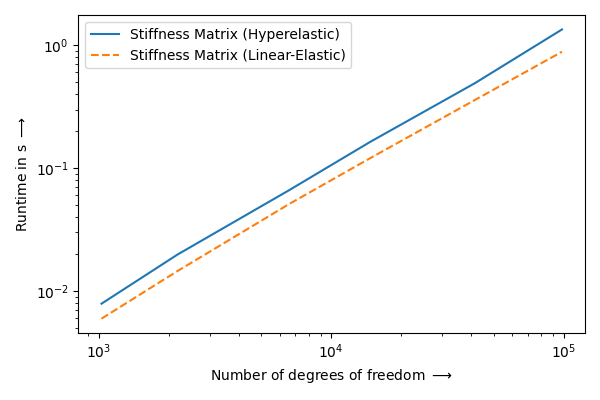
Analysis |
DOF/s |
|---|---|
Linear-Elastic |
136193 +/-22916 |
Hyperelastic |
100613 +/-18702 |
Tested on: Windows 10, Python 3.11, Intel® Core™ i7-11850H @ 2.50GHz, 32GB RAM.
from timeit import timeit

import matplotlib.pyplot as plt
import numpy as np

import felupe as fem


def pre_linear_elastic(n, **kwargs):
   mesh = fem.Cube(n=n).triangulate()
   region = fem.RegionTetra(mesh)
   field = fem.FieldContainer([fem.Field(region, dim=3)])
   umat = fem.LinearElastic(E=1, nu=0.3)
   solid = fem.SolidBody(umat, field)
   return mesh, solid


def pre_hyperelastic(n, **kwargs):
   mesh = fem.Cube(n=n).triangulate()
   region = fem.RegionTetra(mesh)
   field = fem.FieldContainer([fem.Field(region, dim=3)])
   umat = fem.NeoHookeCompressible(mu=1.0, lmbda=2.0)
   solid = fem.SolidBody(umat, field)
   return mesh, solid


print("# Assembly Runtimes")
print("")
print("|   DOF   | Linear-Elastic in s | Hyperelastic in s |")
print("| ------- | ------------------- | ----------------- |")

points_per_axis = np.round((np.logspace(3, 5, 6) / 3)**(1 / 3)).astype(int)

number = 3
parallel = False

runtimes = np.zeros((len(points_per_axis), 2))

for i, n in enumerate(points_per_axis):
   mesh, solid = pre_linear_elastic(n)
   matrix = solid.assemble.matrix(parallel=parallel)
   time_linear_elastic = (
      timeit(lambda: solid.assemble.matrix(parallel=parallel), number=number) / number
   )

   mesh, solid = pre_hyperelastic(n)
   matrix = solid.assemble.matrix(parallel=parallel)
   time_hyperelastic = (
      timeit(lambda: solid.assemble.matrix(parallel=parallel), number=number) / number
   )

   runtimes[i] = time_linear_elastic, time_hyperelastic

   print(
      f"| {mesh.points.size:7d} | {runtimes[i][0]:19.2f} | {runtimes[i][1]:17.2f} |"
   )

dofs_le = points_per_axis ** 3 * 3 / runtimes[:, 0]
dofs_he = points_per_axis ** 3 * 3 / runtimes[:, 1]

print("")
print("| Analysis       |        DOF/s      |")
print("| -------------- | ----------------- |")
print(
   f"| Linear-Elastic |   {np.mean(dofs_le):5.0f} +/-{np.std(dofs_le):5.0f}  |"
)
print(f"| Hyperelastic   |   {np.mean(dofs_he):5.0f} +/-{np.std(dofs_he):5.0f}  |")

plt.figure()
plt.loglog(
   points_per_axis ** 3 * 3,
   runtimes[:, 1],
   "C0",
   label=r"Stiffness Matrix (Hyperelastic)",
)
plt.loglog(
   points_per_axis ** 3 * 3,
   runtimes[:, 0],
   "C1--",
   label=r"Stiffness Matrix (Linear-Elastic)",
)
plt.xlabel(r"Number of degrees of freedom $\longrightarrow$")
plt.ylabel(r"Runtime in s $\longrightarrow$")
plt.legend()
plt.tight_layout()
plt.savefig("benchmark.png")
Contents:
License#
FElupe - Finite Element Analysis (C) 2021-2024 Andreas Dutzler, Graz (Austria).
This program is free software: you can redistribute it and/or modify it under the terms of the GNU General Public License as published by the Free Software Foundation, either version 3 of the License, or (at your option) any later version.
This program is distributed in the hope that it will be useful, but WITHOUT ANY WARRANTY; without even the implied warranty of MERCHANTABILITY or FITNESS FOR A PARTICULAR PURPOSE. See the GNU General Public License for more details.
You should have received a copy of the GNU General Public License along with this program. If not, see https://www.gnu.org/licenses/.