Run a Job

Learn how to apply boundary conditions in a ramped manner within a Step and run a Job.

• create a Step with ramped boundary conditions

• run a Job and export a XDMF time-series file

This tutorial once again covers the essential high-level parts of creating and solving problems with FElupe. This time, however, the external displacements are applied in a ramped manner. The prescribed displacements of a cube under non-homogenous uniaxial loading will be controlled within a step. The Ogden-Roxburgh pseudo-elastic Mullins softening model is combined with an isotropic hyperelastic Neo-Hookean material formulation, which is further applied on a nearly incompressible solid body for a realistic analysis of rubber-like materials. Note that the bulk modulus is now an argument of the (nearly) incompressible solid body instead of the constitutive Neo-Hookean material definition.

import felupe as fem

mesh = fem.Cube(n=6)
region = fem.RegionHexahedron(mesh=mesh)
field = fem.FieldContainer([fem.Field(region=region, dim=3)])

boundaries, loadcase = fem.dof.uniaxial(field, clamped=True)

umat = fem.OgdenRoxburgh(material=fem.NeoHooke(mu=1), r=3, m=1, beta=0)
body = fem.SolidBodyNearlyIncompressible(umat=umat, field=field, bulk=5000)

The ramped prescribed displacements for 12 substeps are created with linsteps(). A Step is created with a list of items to be considered (here, one single solid body) and a dict of ramped boundary conditions along with the prescribed values.

move = fem.math.linsteps([0, 2, 1.5], num=[8, 4])
uniaxial = fem.Step(
    items=[body], ramp={boundaries["move"]: move}, boundaries=boundaries
)

This step is now added to a Job. The results are exported after each completed and successful substep as a time-series XDMF-file. A CharacteristicCurve-job logs the displacement and sum of reaction forces on a given boundary condition.

job = fem.CharacteristicCurve(steps=[uniaxial], boundary=boundaries["move"])
job.evaluate(filename="result.xdmf", verbose=True)

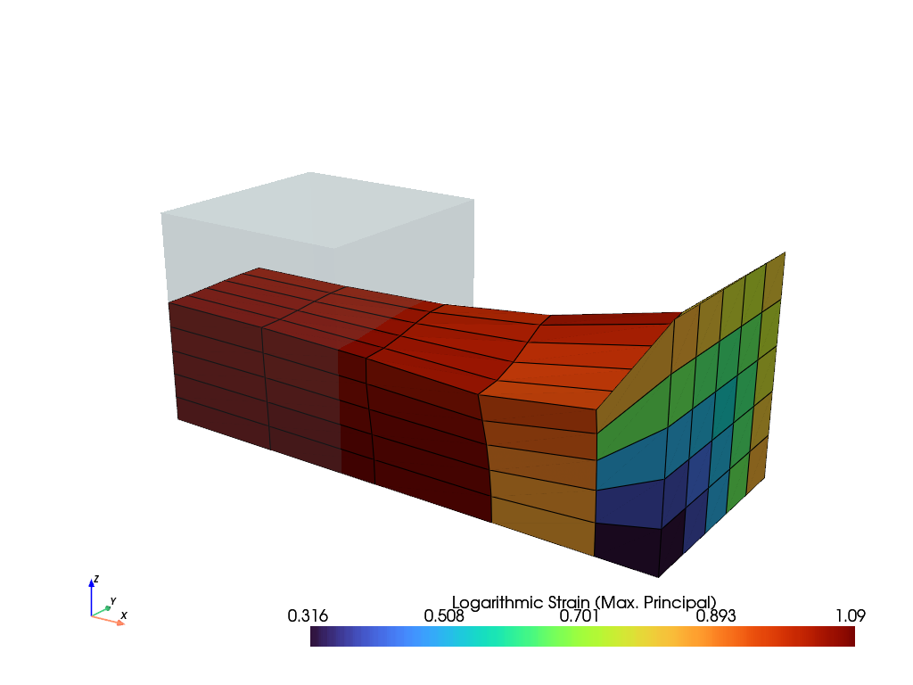
field.plot("Principal Values of Logarithmic Strain").show()

Static Scene

Interactive Scene

  0%|          | 0/13 [00:00<?, ?substep/s]
 15%|█▌        | 2/13 [00:00<00:01,  7.33substep/s]
 23%|██▎       | 3/13 [00:00<00:01,  6.06substep/s]
 31%|███       | 4/13 [00:00<00:01,  5.57substep/s]
 38%|███▊      | 5/13 [00:00<00:01,  5.28substep/s]
 46%|████▌     | 6/13 [00:01<00:01,  5.13substep/s]
 54%|█████▍    | 7/13 [00:01<00:01,  5.04substep/s]
 62%|██████▏   | 8/13 [00:01<00:01,  4.96substep/s]
 69%|██████▉   | 9/13 [00:01<00:00,  4.93substep/s]
 77%|███████▋  | 10/13 [00:02<00:00,  4.06substep/s]
 85%|████████▍ | 11/13 [00:02<00:00,  4.29substep/s]
 92%|█████████▏| 12/13 [00:02<00:00,  4.44substep/s]
100%|██████████| 13/13 [00:02<00:00,  4.56substep/s]
100%|██████████| 13/13 [00:02<00:00,  4.86substep/s]

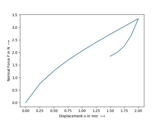
The sum of the reaction force in direction \(x\) on the boundary condition "move" is plotted as a function of the displacement \(u\) on the boundary condition "move" .

fig, ax = job.plot(
    xlabel="Displacement $u$ in mm $\longrightarrow$",
    ylabel="Normal Force $F$ in N $\longrightarrow$",
)

/home/docs/checkouts/readthedocs.org/user_builds/felupe/checkouts/v8.8.0/docs/tutorial/examples/extut02_job.py:2: SyntaxWarning: invalid escape sequence '\l'
  Run a Job
/home/docs/checkouts/readthedocs.org/user_builds/felupe/checkouts/v8.8.0/docs/tutorial/examples/extut02_job.py:3: SyntaxWarning: invalid escape sequence '\l'
  ---------