Run a Job

Learn how to apply boundary conditions in a ramped manner within a Step and run a Job.

• create a Step with ramped boundary conditions

• run a Job and export a XDMF time-series file

This tutorial once again covers the essential high-level parts of creating and solving problems with FElupe. This time, however, the external displacements are applied in a ramped manner. The prescribed displacements of a cube under non-homogenous uniaxial loading will be controlled within a step. The Ogden-Roxburgh pseudo-elastic Mullins softening model is combined with an isotropic hyperelastic Neo-Hookean material formulation, which is further applied on a nearly incompressible solid body for a realistic analysis of rubber-like materials. Note that the bulk modulus is now an argument of the (nearly) incompressible solid body instead of the constitutive Neo-Hookean material definition.

import felupe as fem

mesh = fem.Cube(n=6)
region = fem.RegionHexahedron(mesh=mesh)
field = fem.FieldContainer([fem.Field(region=region, dim=3)])

boundaries = fem.dof.uniaxial(field, clamped=True, return_loadcase=False)

umat = fem.OgdenRoxburgh(material=fem.NeoHooke(mu=1), r=3, m=1, beta=0)
body = fem.SolidBodyNearlyIncompressible(umat=umat, field=field, bulk=5000)

The ramped prescribed displacements for 12 substeps are created with linsteps(). A Step is created with a list of items to be considered (here, one single solid body) and a dict of ramped boundary conditions along with the prescribed values.

move = fem.math.linsteps([0, 2, 1.5], num=[8, 4])
uniaxial = fem.Step(
    items=[body], ramp={boundaries["move"]: move}, boundaries=boundaries
)

This step is now added to a Job. The results are exported after each completed and successful substep as a time-series XDMF-file. A CharacteristicCurve-job logs the displacement and sum of reaction forces on a given boundary condition.

job = fem.CharacteristicCurve(steps=[uniaxial], boundary=boundaries["move"])
job.evaluate(filename="result.xdmf")

field.plot("Principal Values of Logarithmic Strain").show()

Static Scene

Interactive Scene

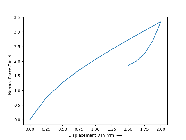
The sum of the reaction force in direction \(x\) on the boundary condition "move" is plotted as a function of the displacement \(u\) on the boundary condition "move" .

fig, ax = job.plot(
    xlabel=r"Displacement $u$ in mm $\longrightarrow$",
    ylabel=r"Normal Force $F$ in N $\longrightarrow$",
)