Hyperelasticity

This page contains hyperelastic material model formulations with automatic differentiation using tensortrax.math. These material model formulations are defined by a strain energy density function.

Differentiable Tensors based on NumPy Arrays.

Frameworks

Hyperelastic(fun[, nstatevars, parallel])

A hyperelastic material definition with a given function for the strain energy density function per unit undeformed volume with Automatic Differentiation provided by tensortrax.

Material Models (Strain Energy Functions) for Hyperelastic

alexander(C, C1, C2, C3, gamma, k)	Strain energy function of the isotropic hyperelastic Alexander material formulation [1]_.
anssari_benam_bucchi(C, mu, N)	Strain energy function of the isotropic hyperelastic generalized Neo-Hookean Anssari-Benam Bucchi material formulation [1]_.
arruda_boyce(C, C1, limit)	Strain energy function of the isotropic hyperelastic Arruda-Boyce material formulation.
extended_tube(C, Gc, delta, Ge, beta)	Strain energy function of the isotropic hyperelastic Extended Tube [1]_ material formulation.
finite_strain_viscoelastic(C, Cin, mu, eta, ...)	Multiplicative finite strain viscoelastic [1]_ material formulation.
lopez_pamies(C, mu, alpha)	Strain energy function of the isotropic hyperelastic Lopez-Pamies material formulation [1]_.
miehe_goektepe_lulei(C, mu, N, U, p, q)	Strain energy function of the isotropic hyperelastic micro-sphere model formulation [1]_.
mooney_rivlin(C, C10, C01)	Strain energy function of the isotropic hyperelastic Mooney-Rivlin material formulation.
neo_hooke(C, mu)	Strain energy function of the isotropic hyperelastic Neo-Hookean material formulation.
ogden(C, mu, alpha)	Strain energy function of the isotropic hyperelastic Ogden material formulation.
ogden_roxburgh(C, Wmax_n, material, r, m, ...)	Ogden-Roxburgh Pseudo-Elastic material formulation for an isotropic treatment of the load-history dependent Mullins-softening of rubber-like materials.
saint_venant_kirchhoff(C, mu, lmbda)	Strain energy function of the isotropic hyperelastic Saint-Venant Kirchhoff material formulation.
third_order_deformation(C, C10, C01, C11, ...)	Strain energy function of the isotropic hyperelastic Third-Order-Deformation material formulation.
van_der_waals(C, mu, limit, a, beta)	Strain energy function of the Van der Waals [1]_ material formulation.,
yeoh(C, C10, C20, C30)	Strain energy function of the isotropic hyperelastic Yeoh material formulation.

Detailed API Reference

class felupe.Hyperelastic(fun, nstatevars=0, parallel=False, **kwargs)

A hyperelastic material definition with a given function for the strain energy density function per unit undeformed volume with Automatic Differentiation provided by tensortrax.

Parameters:

• fun (callable) – A strain energy density function in terms of the right Cauchy-Green deformation tensor \(\boldsymbol{C}\). Function signature must be fun = lambda C, **kwargs: psi for functions without state variables and fun = lambda C, statevars, **kwargs: [psi, statevars_new] for functions with state variables. The right Cauchy-Green deformation tensor will be a tensortrax.Tensor when the function is evaluated. It is important to only use differentiable math-functions from tensortrax.math.

• nstatevars (int, optional) – Number of state variables (default is 0).

• parallel (bool, optional) – A flag to invoke threaded strain energy density function evaluations (default is False). May introduce additional overhead for small-sized problems.

• **kwargs (dict, optional) – Optional keyword-arguments for the strain energy density function.

Notes

The strain energy density function \(\psi\) must be given in terms of the right Cauchy-Green deformation tensor \(\boldsymbol{C} = \boldsymbol{F}^T \boldsymbol{F}\).

Warning

It is important to only use differentiable math-functions from tensortrax.math!

Take this minimal code-block as template

\[\psi = \psi(\boldsymbol{C})\]

import tensortrax.math as tm

def neo_hooke(C, mu):
    "Strain energy function of the Neo-Hookean material formulation."
    return mu / 2 * (tm.linalg.det(C) ** (-1/3) * tm.trace(C) - 3)

umat = fem.Hyperelastic(neo_hooke, mu=1)

and this code-block for material formulations with state variables.

\[\psi = \psi(\boldsymbol{C}, \boldsymbol{\zeta})\]

import tensortrax.math as tm

def viscoelastic(C, Cin, mu, eta, dtime):
    "Finite strain viscoelastic material formulation."

    # unimodular part of the right Cauchy-Green deformation tensor
    Cu = tm.linalg.det(C) ** (-1 / 3) * C

    # update of state variables by evolution equation
    Ci = tm.special.from_triu_1d(Cin, like=C) + mu / eta * dtime * Cu
    Ci = tm.linalg.det(Ci) ** (-1 / 3) * Ci

    # first invariant of elastic part of right Cauchy-Green deformation tensor
    I1 = tm.trace(Cu @ tm.linalg.inv(Ci))

    # strain energy function and state variable
    return mu / 2 * (I1 - 3), tm.special.triu_1d(Ci)

umat = fem.Hyperelastic(
    viscoelastic, mu=1, eta=1, dtime=1, nstatevars=6
)

Note

See the documentation of tensortrax for further details.

Examples

View force-stretch curves on elementary incompressible deformations.

>>> import felupe as fem
>>> import tensortrax.math as tm
>>>
>>> def neo_hooke(C, mu):
...     "Strain energy function of the Neo-Hookean material formulation."
...     return mu / 2 * (tm.linalg.det(C) ** (-1/3) * tm.trace(C) - 3)
>>>
>>> umat = fem.Hyperelastic(neo_hooke, mu=1)
>>> ax = umat.plot(incompressible=True)

See also

saint_venant_kirchhoff

Strain energy function of the Saint Venant-Kirchhoff material formulation.

neo_hooke

Strain energy function of the Neo-Hookean material formulation.

mooney_rivlin

Strain energy function of the Mooney-Rivlin material formulation.

yeoh

“Strain energy function of the Yeoh material formulation.

third_order_deformation

Strain energy function of the Third-Order-Deformation material formulation.

ogden

Strain energy function of the Ogden material formulation.

arruda_boyce

Strain energy function of the Arruda-Boyce material formulation.

extended_tube

Strain energy function of the Extended-Tube material formulation.

van_der_waals

Strain energy function of the Van der Waals material formulation.

finite_strain_viscoelastic

Finite strain viscoelastic material formulation.

copy()

Return a deep-copy of the constitutive material.

gradient(x)

Return the evaluated gradient of the strain energy density function.

Parameters:

x (list of ndarray) – The list with input arguments. These contain the extracted fields of a FieldContainer along with the old vector of state variables, [*field.extract(), statevars_old].

Returns:

A list with the evaluated gradient(s) of the strain energy density function and the updated vector of state variables.

Return type:

list of ndarray

hessian(x)

Return the evaluated upper-triangle components of the hessian(s) of the strain energy density function.

Parameters:

x (list of ndarray) – The list with input arguments. These contain the extracted fields of a FieldContainer along with the old vector of state variables, [*field.extract(), statevars_old].

Returns:

A list with the evaluated upper-triangle components of the hessian(s) of the strain energy density function.

Return type:

list of ndarray

optimize(ux=None, ps=None, bx=None, incompressible=False, relative=False, **kwargs)

Optimize the material parameters by a least-squares fit on experimental stretch-stress data.

Parameters:

• ux (array of shape (2, ...) or None, optional) – Experimental uniaxial stretch and force-per-undeformed-area data (default is None).

• ps (array of shape (2, ...) or None, optional) – Experimental planar-shear stretch and force-per-undeformed-area data (default is None).

• bx (array of shape (2, ...) or None, optional) – Experimental biaxial stretch and force-per-undeformed-area data (default is None).

• incompressible (bool, optional) – A flag to enforce incompressible deformations (default is False).

• relative (bool, optional) – A flag to optimize relative instead of absolute residuals, i.e. (predicted - observed) / observed instead of predicted - observed (default is False).

• **kwargs (dict, optional) – Optional keyword arguments are passed to scipy.optimize.least_squares().

Returns:

• ConstitutiveMaterial – A copy of the constitutive material with the optimized material parameters.

• scipy.optimize.OptimizeResult – Represents the optimization result.

Notes

Warning

At least one load case, i.e. one of the arguments ux, ps or bx must not be None.

The vector of residuals is given in Eq. (3) in case of absolute residuals

(1)\[ \begin{align}\begin{aligned}\begin{split}\boldsymbol{r} &= \begin{bmatrix} \boldsymbol{r}_\text{ux} \\ \boldsymbol{r}_\text{ps} \\ \boldsymbol{r}_\text{bx} \end{bmatrix}\end{split}\\r_\text{ux}(\lambda_i) &= P_\text{ux}(\lambda_i) - P_\text{ux, observed}(\lambda_i)\\r_\text{ps}(\lambda_i) &= P_\text{ps}(\lambda_i) - P_\text{ps, observed}(\lambda_i)\\r_\text{bx}(\lambda_i) &= P_\text{bx}(\lambda_i) - P_\text{bx, observed}(\lambda_i)\end{aligned}\end{align} \]

and in Eq. (4) in case of relative residuals.

(2)\[ \begin{align}\begin{aligned}\begin{split}\boldsymbol{r} &= \begin{bmatrix} \boldsymbol{r}_\text{ux} \\ \boldsymbol{r}_\text{ps} \\ \boldsymbol{r}_\text{bx} \end{bmatrix}\end{split}\\r_\text{ux}(\lambda_i) &= \frac{ P_\text{ux}(\lambda_i) - P_\text{ux, observed}(\lambda_i)}{ P_\text{ux, observed}(\lambda_i) }\\r_\text{ps}(\lambda_i) &= \frac{ P_\text{ps}(\lambda_i) - P_\text{ps, observed}(\lambda_i)}{ P_\text{ps, observed}(\lambda_i) }\\r_\text{bx}(\lambda_i) &= \frac{ P_\text{bx}(\lambda_i) - P_\text{bx, observed}(\lambda_i)}{ P_\text{bx, observed}(\lambda_i) }\end{aligned}\end{align} \]

Examples

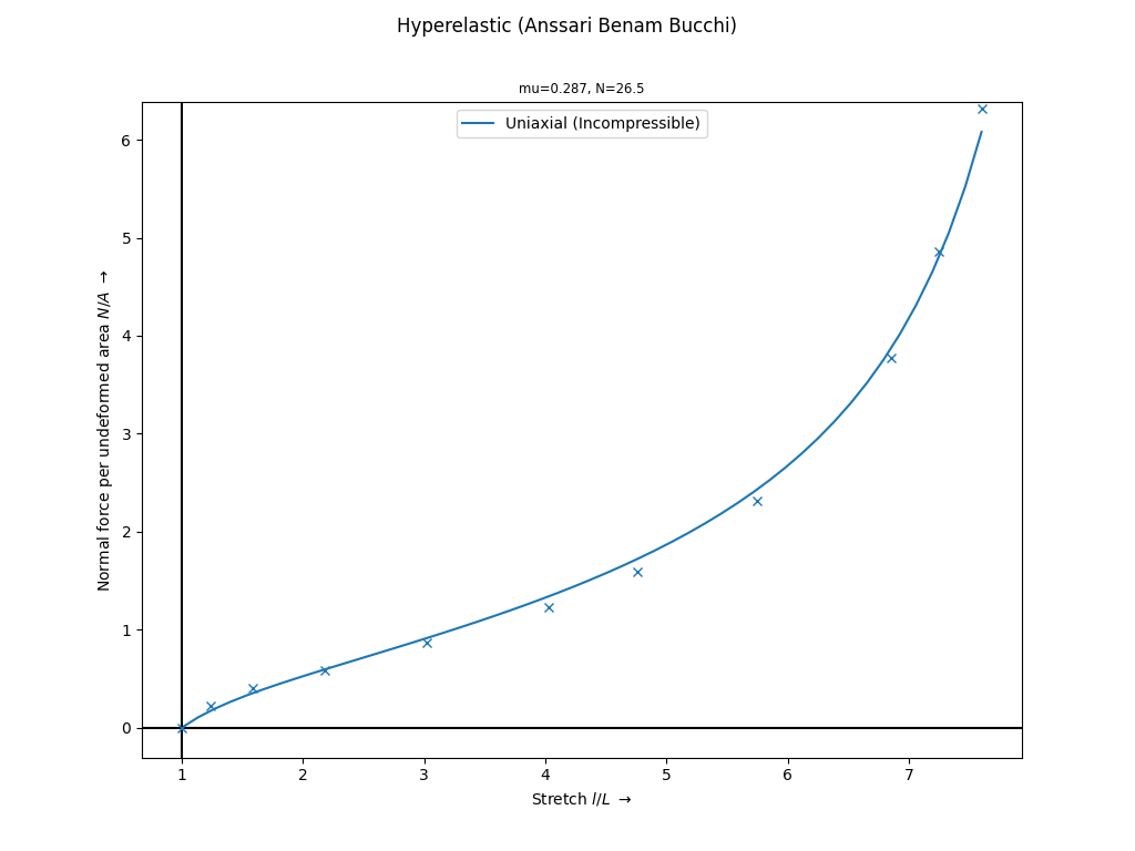
The Anssari-Benam Bucchi material model formulation is best-fitted on Treloar’s uniaxial and biaxial tension data [1]_.

>>> import numpy as np
>>> import felupe as fem
>>>
>>> λ, P = np.array(
...     [
...         [1.000, 0.00],
...         [1.240, 2.30],
...         [1.585, 4.16],
...         [2.180, 6.00],
...         [3.020, 8.80],
...         [4.030, 12.5],
...         [4.760, 16.2],
...         [5.750, 23.6],
...         [6.850, 38.5],
...         [7.250, 49.6],
...         [7.600, 64.4],
...     ]
... ).T * np.array([[1.0], [0.0980665]])
>>>
>>> umat = fem.Hyperelastic(fem.anssari_benam_bucchi)
>>> umat_new, res = umat.optimize(
...     ux=[λ, P], incompressible=True, relative=True
... )
>>>
>>> ux = np.linspace(λ.min(), λ.max(), num=50)
>>> ax = umat_new.plot(incompressible=True, ux=ux, bx=None, ps=None)

>>> ax.plot(λ, P, "C0x")

See also

scipy.optimize.least_squares

Solve a nonlinear least-squares problem with bounds on the variables.

References

[1]

L. R. G. Treloar, “Stress-strain data for vulcanised rubber under various types of deformation”, Transactions of the Faraday Society, vol. 40. Royal Society of Chemistry (RSC), p. 59, 1944. doi: 10.1039/tf9444000059. Data available at https://www.uni-due.de/mathematik/ag_neff/neff_hencky.

plot(incompressible=False, **kwargs)

Return a plot with normal force per undeformed area vs. stretch curves for the elementary homogeneous deformations uniaxial tension/compression, planar shear and biaxial tension of a given isotropic material formulation.

Parameters:

• incompressible (bool, optional) – A flag to enforce views on incompressible deformations (default is False).

• **kwargs (dict, optional) – Optional keyword-arguments for ViewMaterial or ViewMaterialIncompressible.

Return type:

matplotlib.axes.Axes

See also

felupe.ViewMaterial

Create views on normal force per undeformed area vs. stretch curves for the elementary homogeneous deformations uniaxial tension/compression, planar shear and biaxial tension of a given isotropic material formulation.

felupe.ViewMaterialIncompressible

Create views on normal force per undeformed area vs. stretch curves for the elementary homogeneous incompressible deformations uniaxial tension/compression, planar shear and biaxial tension of a given isotropic material formulation.

screenshot(filename='umat.png', incompressible=False, **kwargs)

Save a screenshot with normal force per undeformed area vs. stretch curves for the elementary homogeneous deformations uniaxial tension/compression, planar shear and biaxial tension of a given isotropic material formulation.

Parameters:

• filename (str, optional) – The filename of the screenshot (default is “umat.png”).

• incompressible (bool, optional) – A flag to enforce views on incompressible deformations (default is False).

• **kwargs (dict, optional) – Optional keyword-arguments for ViewMaterial or ViewMaterialIncompressible.

Return type:

matplotlib.axes.Axes

See also

felupe.ViewMaterial

Create views on normal force per undeformed area vs. stretch curves for the elementary homogeneous deformations uniaxial tension/compression, planar shear and biaxial tension of a given isotropic material formulation.

felupe.ViewMaterialIncompressible

Create views on normal force per undeformed area vs. stretch curves for the elementary homogeneous incompressible deformations uniaxial tension/compression, planar shear and biaxial tension of a given isotropic material formulation.

view(incompressible=False, **kwargs)

Create views on normal force per undeformed area vs. stretch curves for the elementary homogeneous deformations uniaxial tension/compression, planar shear and biaxial tension of a given isotropic material formulation.

Parameters:

• incompressible (bool, optional) – A flag to enforce views on incompressible deformations (default is False).

• **kwargs (dict, optional) – Optional keyword-arguments for ViewMaterial or ViewMaterialIncompressible.

Return type:

felupe.ViewMaterial or felupe.ViewMaterialIncompressible

See also

felupe.ViewMaterial

Create views on normal force per undeformed area vs. stretch curves for the elementary homogeneous deformations uniaxial tension/compression, planar shear and biaxial tension of a given isotropic material formulation.

felupe.ViewMaterialIncompressible

Create views on normal force per undeformed area vs. stretch curves for the elementary homogeneous incompressible deformations uniaxial tension/compression, planar shear and biaxial tension of a given isotropic material formulation.

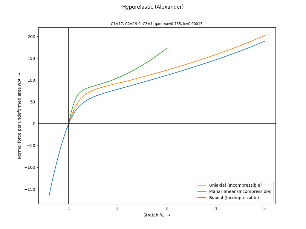
felupe.alexander(C, C1, C2, C3, gamma, k)

Strain energy function of the isotropic hyperelastic Alexander material formulation [1]_.

Parameters:

• C (tensortrax.Tensor) – Right Cauchy-Green deformation tensor.

• C1 (float) – Scale factor for the first invariant term.

• C2 (float) – Scale factor for the second invariant term.

• C3 (float) – Scale factor for the logarithmic second invariant term.

• gamma (float) – Offset-normalization parameter for the logarithmic second invariant term.

• k (float) – Scale factor for the exponential first invariant term.

Notes

Warning

The strain energy function of the Alexander model formulation is not directly implemented. Only its gradient and hessian w.r.t. the right Cauchy-Green deformation tensor are defined. This is because the imaginary error-function \(\text{erfi}(x)\) is not included in NumPy - this would require SciPy as a dependency.

The strain energy function is given in Eq. (3)

(3)\[\psi = C_1 \int_{\hat{I}_1} \exp \left( k \left(\hat{I}_1 - 3 \right)^2 \right) \ d\hat{I}_1 + C_2 \ln \left(\frac{\hat{I}_2 - 3 + \gamma}{\gamma} \right) + C_3 \left(\hat{I}_2 - 3 \right)\]

with the first and second main invariant of the distortional part of the right Cauchy-Green deformation tensor, see Eq. (4).

(4)\[ \begin{align}\begin{aligned}\hat{I}_1 &= J^{-2/3} \text{tr}\left( \boldsymbol{C} \right)\\\hat{I}_2 &= J^{-4/3} \frac{1}{2} \left( \text{tr}\left(\boldsymbol{C}\right)^2 - \text{tr}\left(\boldsymbol{C}^2\right) \right)\end{aligned}\end{align} \]

The initial shear modulus \(\mu\) is given in Eq. (5).

(5)\[\mu = 2 \left( C_1 + \frac{C_2}{\gamma} + C_3 \right)\]

Examples

>>> import felupe as fem
>>>
>>> umat = fem.Hyperelastic(
...    fem.alexander, C1=17, C2=19.85, C3=1, gamma=0.735, k=0.00015
... )
>>> ux = fem.math.linsteps([0.6, 5], num=50)
>>> ps = fem.math.linsteps([1, 5], num=50)
>>> bx = fem.math.linsteps([1, 3], num=50)
>>>
>>> ax = umat.plot(ux=ux, ps=ps, bx=bx, incompressible=True)

References

[1]

H. Alexander, “A constitutive relation for rubber-like materials”, International Journal of Engineering Science, vol. 6, no. 9. Elsevier BV, pp. 549–563, Sep. 1968. doi: 10.1016/0020-7225(68)90006-2.

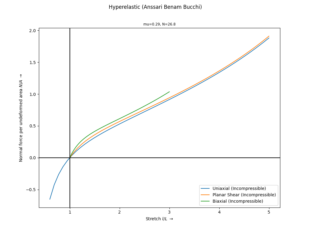
felupe.anssari_benam_bucchi(C, mu, N)

Strain energy function of the isotropic hyperelastic generalized Neo-Hookean Anssari-Benam Bucchi material formulation [1]_.

Parameters:

• C (tensortrax.Tensor) – Right Cauchy-Green deformation tensor.

• mu (float) – Modulus \(\mu = nkT\) - this is not the infinitesimal shear modulus.

• N (float) – Number of Kuhn segments of a chain.

Notes

The strain energy function is given in Eq. (6)

(6)\[\psi = \mu N \left( \frac{1}{6N} \left( \hat{I}_1 - 3 \right) - \ln \left( \frac{\hat{I}_1 - 3N}{3 - 3N} \right) \right)\]

with the first main invariant of the distortional part of the right Cauchy-Green deformation tensor, see Eq. (7).

(7)\[\hat{I}_1 = J^{-2/3} \text{tr}\left( \boldsymbol{C} \right)\]

The initial shear modulus \(\mu_0\) is given in Eq. (8).

(8)\[\mu_0 = \mu \frac{1 - 3N}{3 - 3N}\]

Examples

>>> import felupe as fem
>>>
>>> umat = fem.Hyperelastic(fem.anssari_benam_bucchi, mu=0.29, N=26.8)
>>>
>>> ux = fem.math.linsteps([0.6, 5], num=50)
>>> ps = fem.math.linsteps([1, 5], num=50)
>>> bx = fem.math.linsteps([1, 3], num=50)
>>>
>>> ax = umat.plot(ux=ux, ps=ps, bx=bx, incompressible=True)

References

[1]

A. Anssari-Benam and A. Bucchi, “A generalised neo-Hookean strain energy function for application to the finite deformation of elastomers”, International Journal of Non-Linear Mechanics, vol. 128. Elsevier BV, p. 103626, Jan. 2021. doi: 10.1016/j.ijnonlinmec.2020.103626.

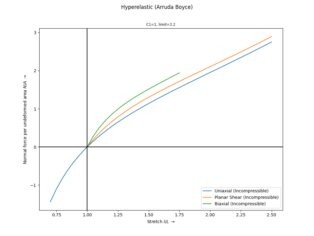
felupe.arruda_boyce(C, C1, limit)

Strain energy function of the isotropic hyperelastic Arruda-Boyce material formulation.

Parameters:

• C (tensortrax.Tensor) – Right Cauchy-Green deformation tensor.

• C1 (float) – Initial shear modulus.

• limit (float) – Limiting stretch \(\lambda_m\) at which the polymer chain network becomes locked.

Notes

The strain energy function is given in Eq. (9)

(9)\[\psi = C_1 \sum_{i=1}^5 \alpha_i \beta^{i-1} \left( \hat{I}_1^i - 3^i \right)\]

with the first main invariant of the distortional part of the right Cauchy-Green deformation tensor as given in Eq. (10)

(10)\[\hat{I}_1 = J^{-2/3} \text{tr}\left( \boldsymbol{C} \right)\]

and \(\alpha_i\) and \(\beta\) as denoted in Eq. (11).

(11)\[ \begin{align}\begin{aligned}\begin{split}\boldsymbol{\alpha} &= \begin{bmatrix} \frac{1}{2} \\ \frac{1}{20} \\ \frac{11}{1050} \\ \frac{19}{7000} \\ \frac{519}{673750} \end{bmatrix}\end{split}\\\beta &= \frac{1}{\lambda_m^2}\end{aligned}\end{align} \]

The initial shear modulus is a function of both material parameters, see Eq. (12).

(12)\[\mu = C_1 \left( 1 + \frac{3}{5 \lambda_m^2} + \frac{99}{175 \lambda_m^4} + \frac{513}{875 \lambda_m^6} + \frac{42039}{67375 \lambda_m^8} \right)\]

Examples

>>> import felupe as fem
>>>
>>> umat = fem.Hyperelastic(fem.arruda_boyce, C1=1.0, limit=3.2)
>>> ax = umat.plot(incompressible=True)

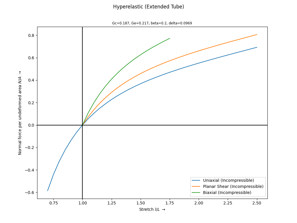
felupe.extended_tube(C, Gc, delta, Ge, beta)

Strain energy function of the isotropic hyperelastic Extended Tube [1]_ material formulation.

Parameters:

• C (tensortrax.Tensor) – Right Cauchy-Green deformation tensor.

• Gc (float) – Cross-link contribution to the initial shear modulus.

• delta (float) – Finite extension parameter of the polymer strands.

• Ge (float) – Constraint contribution to the initial shear modulus.

• beta (float) – Global rearrangements of cross-links upon deformation (release of topological constraints).

Notes

The strain energy function is given in Eq. (13)

(13)\[\psi = \frac{G_c}{2} \left[ \frac{\left( 1 - \delta^2 \right) \left( \hat{I}_1 - 3 \right)}{1 - \delta^2 \left( \hat{I}_1 - 3 \right)} + \ln \left( 1 - \delta^2 \left( \hat{I}_1 - 3 \right) \right) \right] + \frac{2 G_e}{\beta^2} \left( \hat{\lambda}_1^{-\beta} + \hat{\lambda}_2^{-\beta} + \hat{\lambda}_3^{-\beta} - 3 \right)\]

with the first main invariant of the distortional part of the right Cauchy-Green deformation tensor as given in Eq. (14)

(14)\[\hat{I}_1 = J^{-2/3} \text{tr}\left( \boldsymbol{C} \right)\]

and the principal stretches, obtained from the distortional part of the right Cauchy-Green deformation tensor, see Eq. (15).

(15)\[ \begin{align}\begin{aligned}\lambda^2_\alpha &= \text{eigvals}\left( \boldsymbol{C} \right)\\\hat{\lambda}_\alpha &= J^{-1/3} \lambda_\alpha\end{aligned}\end{align} \]

The initial shear modulus results from the sum of the cross-link and the constraint contributions to the total initial shear modulus as denoted in Eq. (16).

(16)\[\mu = G_e + G_c\]

Examples

>>> import felupe as fem
>>>
>>> umat = fem.Hyperelastic(
...     fem.extended_tube, Gc=0.1867, Ge=0.2169, beta=0.2, delta=0.09693
... )
>>> ax = umat.plot(incompressible=True)

References

[1]

M. Kaliske and G. Heinrich, “An Extended Tube-Model for Rubber Elasticity: Statistical-Mechanical Theory and Finite Element Implementation”, Rubber Chemistry and Technology, vol. 72, no. 4. Rubber Division, ACS, pp. 602–632, Sep. 01, 1999. doi: 10.5254/1.3538822.

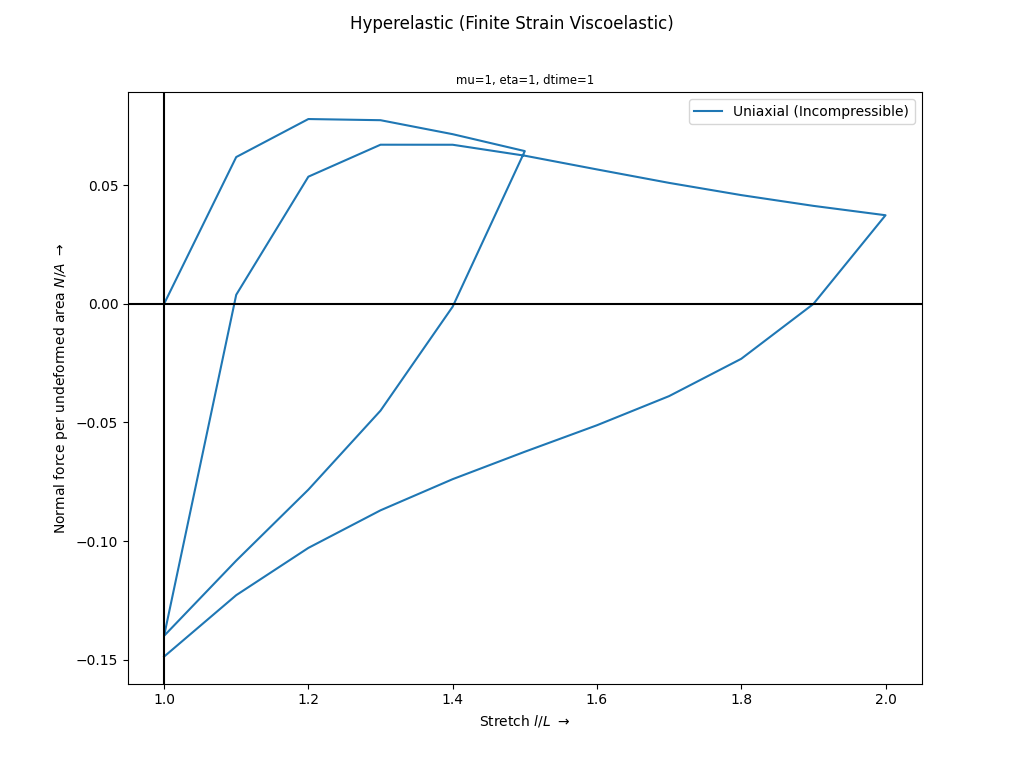
felupe.finite_strain_viscoelastic(C, Cin, mu, eta, dtime)

Multiplicative finite strain viscoelastic [1]_ material formulation.

Notes

The material formulation is built upon the multiplicative decomposition of the distortional part of the deformation gradient tensor into an elastic and an inelastic part, see Eq. (17).

(17)\[ \begin{align}\begin{aligned}\hat{\boldsymbol{F}} &= \boldsymbol{F}_e \boldsymbol{F}_i \ (= \hat{\boldsymbol{F}_e} \boldsymbol{F}_i)\\\boldsymbol{C}_e &= \boldsymbol{F}_e^T \boldsymbol{F}_e\\\boldsymbol{C}_i &= \boldsymbol{F}_i^T \boldsymbol{F}_i\\\text{tr}\left( \boldsymbol{C}_e \right) &= \text{tr}\left( \hat{\boldsymbol{C}} \boldsymbol{C}_i^{-1} \right)\end{aligned}\end{align} \]

The components of the inelastic right Cauchy-Green deformation tensor are used as state variables with the evolution equation and its explicit update formula as given in Eq. (18) [1]_. The elastic part of the multiplicative decomposition of the deformation gradient tensor is also enforced to be an unimodular tensor which leads to the constraint \(\det(\boldsymbol{F_i})=1\). Hence, the inelastic right Cauchy-Green deformation tensor must be an unimodular tensor \(\det(\boldsymbol{C_i})=1\).

(18)\[ \begin{align}\begin{aligned}\dot{\boldsymbol{C}}_i &= \frac{\mu}{\eta}\ \hat{\boldsymbol{C}}\\\boldsymbol{C}_i &= \hat{\overline{\boldsymbol{C}_{i,n} + \frac{\Delta t \mu}{\eta} \hat{\boldsymbol{C}}}}\end{aligned}\end{align} \]

The distortional part of the strain energy density per unit undeformed volume is assumed to be of a Neo-Hookean form, see Eq. (19).

(19)\[\hat{\psi} = \frac{\mu}{2} \left( \text{tr}\left( \hat{\boldsymbol{C}} \boldsymbol{C}_i^{-1} \right) - 3 \right)\]

Examples

>>> import felupe as fem
>>>
>>> umat = fem.Hyperelastic(
...     fem.finite_strain_viscoelastic, mu=1.0, eta=1.0, dtime=1.0, nstatevars=6
... )
>>> ax = umat.plot(
...    incompressible=True,
...    ux=fem.math.linsteps([1, 1.5, 1, 2, 1], num=[5, 5, 10, 10]),
...    ps=None,
...    bx=None,
... )

References

[1]

A. V. Shutov, R. Landgraf, and J. Ihlemann, “An explicit solution for implicit time stepping in multiplicative finite strain viscoelasticity”, Computer Methods in Applied Mechanics and Engineering, vol. 265. Elsevier BV, pp. 213–225, Oct. 2013. doi: 10.1016/j.cma.2013.07.004.

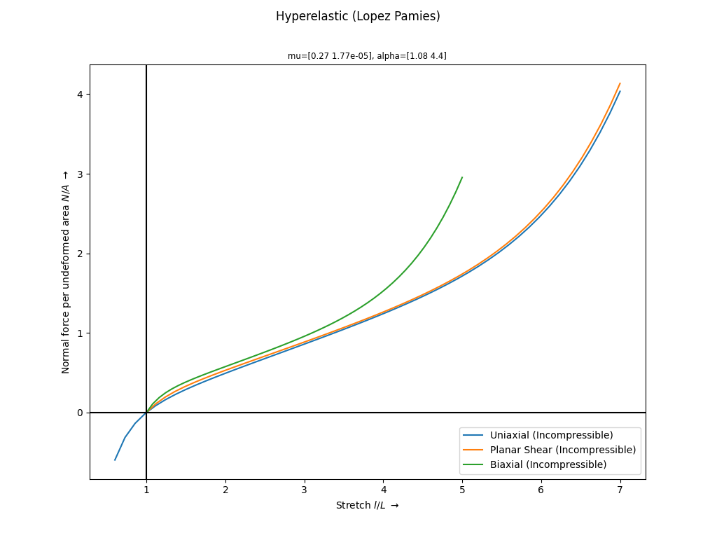
felupe.lopez_pamies(C, mu, alpha)

Strain energy function of the isotropic hyperelastic Lopez-Pamies material formulation [1]_.

Parameters:

• C (tensortrax.Tensor) – Right Cauchy-Green deformation tensor.

• mu (list of float) – List of moduli.

• alpha (list of float) – List of invariant exponents.

Notes

The strain energy function is given in Eq. (20)

(20)\[\psi = \sum_{r=1}^M \frac{3^{1-\alpha_r}}{2 \alpha_r} \mu_r \left( \hat{I}_1^{\alpha_r} - 3^{\alpha_r} \right)\]

with the first main invariant of the distortional part of the right Cauchy-Green deformation tensor, see Eq. (21).

(21)\[\hat{I}_1 = J^{-2/3} \text{tr}\left( \boldsymbol{C} \right)\]

The sum of the moduli \(\mu_r\) is equal to the initial shear modulus \(\mu\), see Eq. (22).

(22)\[\mu = \sum_r \mu_r\]

Examples

>>> import felupe as fem
>>>
>>> umat = fem.Hyperelastic(
...     fem.lopez_pamies, mu=[0.2699,  0.00001771], alpha=[1.08, 4.40]
... )
>>>
>>> ux = fem.math.linsteps([0.6, 7], num=50)
>>> ps = fem.math.linsteps([1, 7], num=50)
>>> bx = fem.math.linsteps([1, 5], num=50)
>>>
>>> ax = umat.plot(ux=ux, ps=ps, bx=bx, incompressible=True)

References

[1]

O. Lopez-Pamies, “A new I1-based hyperelastic model for rubber elastic materials”, Comptes Rendus. Mécanique, vol. 338, no. 1. Cellule MathDoc/Centre Mersenne, pp. 3–11, Dec. 23, 2009. doi: 10.1016/j.crme.2009.12.007.

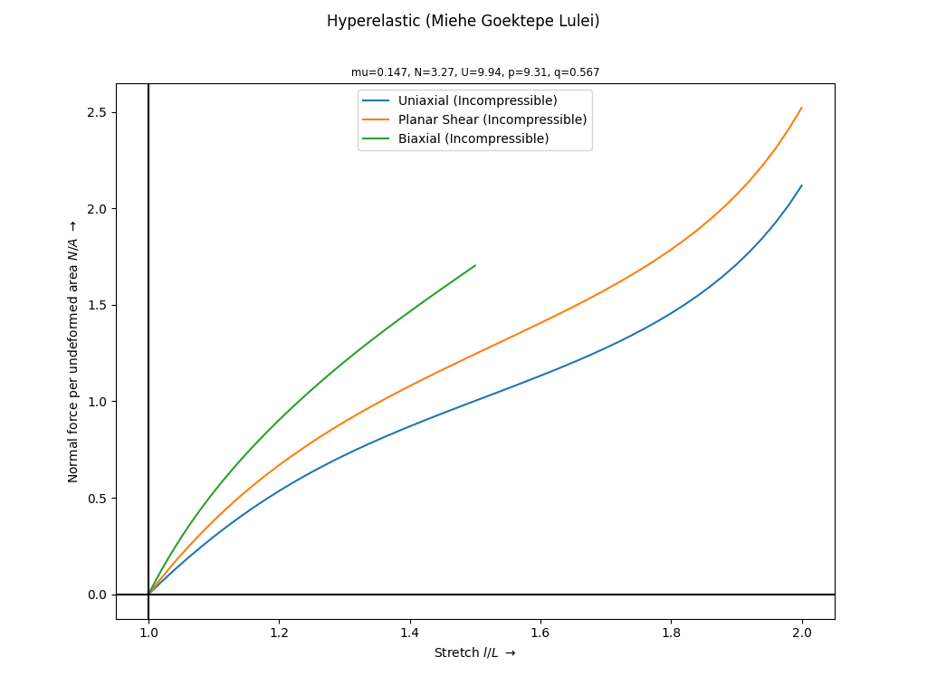
felupe.miehe_goektepe_lulei(C, mu, N, U, p, q)

Strain energy function of the isotropic hyperelastic micro-sphere model formulation [1]_.

Parameters:

• C (tensortrax.Tensor) – Right Cauchy-Green deformation tensor.

• mu (float) – Shear modulus (ground state stifness).

• N (float) – Number of chain segments (chain locking response).

• U (float) – Tube geometry parameter (3D locking characteristics).

• p (float) – Non-affine stretch parameter (additional constraint stifness).

• q (float) – Non-affine tube parameter (shape of constraint stress).

Examples

>>> import felupe as fem
>>>
>>> umat = fem.Hyperelastic(
...     fem.miehe_goektepe_lulei,
...     mu=0.1475,
...     N=3.273,
...     p=9.31,
...     U=9.94,
...     q=0.567,
... )
>>> ux = ps = fem.math.linsteps([1, 2], num=50)
>>> bx = fem.math.linsteps([1, 1.5], num=50)
>>> ax = umat.plot(ux=ux, ps=ps, bx=bx, incompressible=True)

References

[1]

C. Miehe, S. Göktepe and F. Lulei, “A micro-macro approach to rubber-like materials - Part I: the non-affine micro-sphere model of rubber elasticity”, Journal of the Mechanics and Physics of Solids, vol. 52, no. 11. Elsevier BV, pp. 2617–2660, Nov. 2004. doi: 10.1016/j.jmps.2004.03.011.

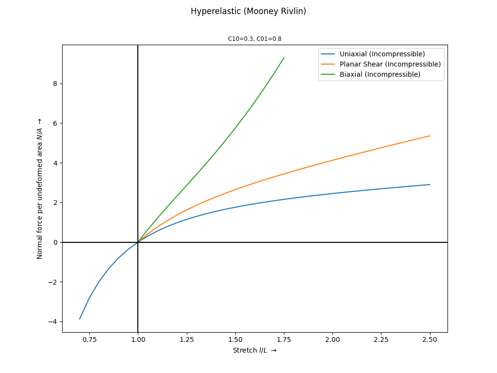
felupe.mooney_rivlin(C, C10, C01)

Strain energy function of the isotropic hyperelastic Mooney-Rivlin material formulation.

Parameters:

• C (tensortrax.Tensor) – Right Cauchy-Green deformation tensor.

• C10 (float) – First material parameter associated to the first invariant.

• C01 (float) – Second material parameter associated to the second invariant.

Notes

The strain energy function is given in Eq. (23)

(23)\[\psi = C_{10} \left(\hat{I}_1 - 3 \right) + C_{01} \left(\hat{I}_2 - 3 \right)\]

with the first and second main invariant of the distortional part of the right Cauchy-Green deformation tensor, see Eq. (24).

(24)\[ \begin{align}\begin{aligned}\hat{I}_1 &= J^{-2/3} \text{tr}\left( \boldsymbol{C} \right)\\\hat{I}_2 &= J^{-4/3} \frac{1}{2} \left( \text{tr}\left(\boldsymbol{C}\right)^2 - \text{tr}\left(\boldsymbol{C}^2\right) \right)\end{aligned}\end{align} \]

The doubled sum of both material parameters is equal to the shear modulus \(\mu\) as denoted in Eq. (25).

(25)\[\mu = 2 \left( C_{10} + C_{01} \right)\]

Examples

>>> import felupe as fem
>>>
>>> umat = fem.Hyperelastic(fem.mooney_rivlin, C10=0.3, C01=0.8)
>>> ax = umat.plot(incompressible=True)

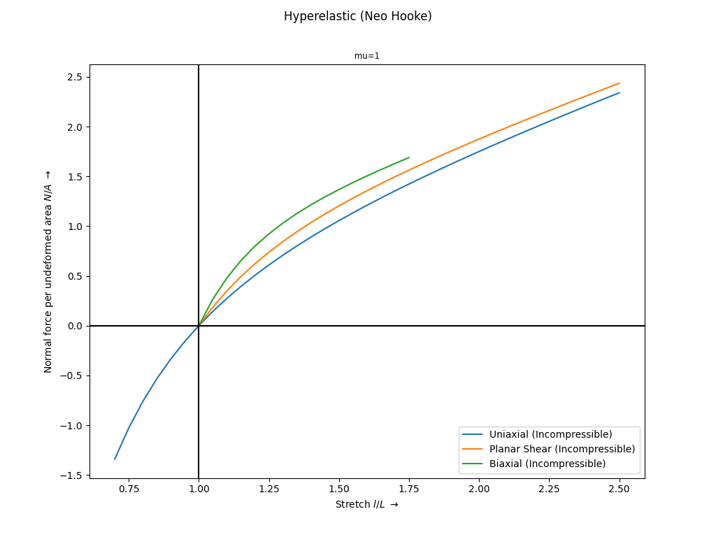
felupe.neo_hooke(C, mu)

Strain energy function of the isotropic hyperelastic Neo-Hookean material formulation.

Parameters:

• C (tensortrax.Tensor) – Right Cauchy-Green deformation tensor.

• mu (float) – Shear modulus.

Notes

The strain energy function is given in Eq. (26).

(26)\[\psi = \frac{\mu}{2} \left(\text{tr}\left(\hat{\boldsymbol{C}}\right) - 3\right)\]

Examples

>>> import felupe as fem
>>>
>>> umat = fem.Hyperelastic(fem.neo_hooke, mu=1.0)
>>> ax = umat.plot(incompressible=True)

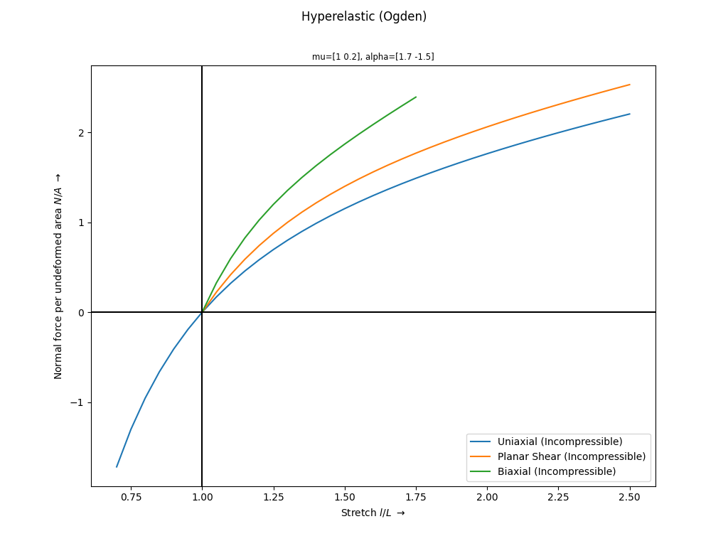
felupe.ogden(C, mu, alpha)

Strain energy function of the isotropic hyperelastic Ogden material formulation.

Parameters:

• C (tensortrax.Tensor) – Right Cauchy-Green deformation tensor.

• mu (list of float) – List of moduli.

• alpha (list of float) – List of stretch exponents.

Notes

The strain energy function is given in Eq. (27)

(27)\[\psi = \sum_i \frac{2 \mu_i}{\alpha^2_i} \left( \lambda_1^{\alpha_i} + \lambda_2^{\alpha_i} + \lambda_3^{\alpha_i} - 3 \right)\]

The sum of the moduli \(\mu_i\) is equal to the initial shear modulus \(\mu\), see Eq. (28).

(28)\[\mu = \sum_i \mu_i\]

Examples

>>> import felupe as fem
>>>
>>> umat = fem.Hyperelastic(fem.ogden, mu=[1, 0.2], alpha=[1.7, -1.5])
>>> ax = umat.plot(incompressible=True)

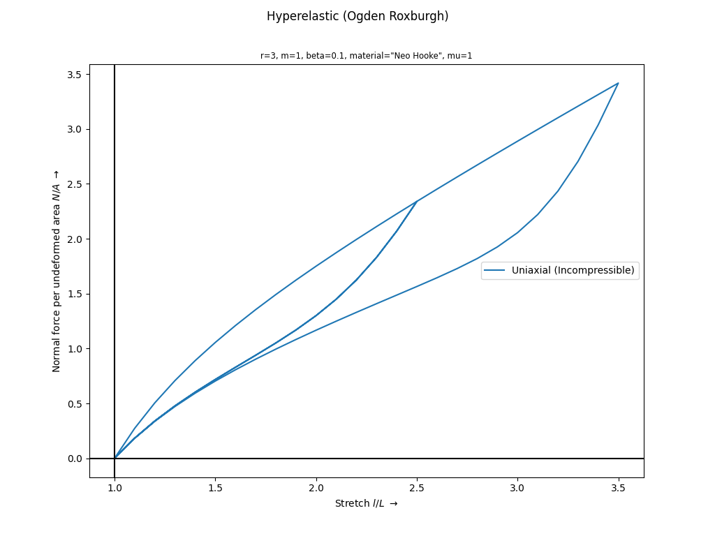
felupe.ogden_roxburgh(C, Wmax_n, material, r, m, beta, **kwargs)

Ogden-Roxburgh Pseudo-Elastic material formulation for an isotropic treatment of the load-history dependent Mullins-softening of rubber-like materials.

Parameters:

• C (tensortrax.Tensor) – Right Cauchy-Green deformation tensor.

• Wmax_n (ndarray) – State variable: value of the maximum strain energy density in load-history from the previous solution.

• material (callable) – Isotropic strain-energy density function. Optional keyword arguments are passed to material.

• r (float) – Reciprocal value of the maximum relative amount of softening. i.e. r=3 means the shear modulus of the base material scales down from \(1\) (no softening) to \(1 - 1/3 = 2/3\) (maximum softening).

• m (float) – The initial Mullins softening modulus.

• beta (float) – Maximum deformation-dependent part of the Mullins softening modulus.

• **kwargs (dict) – Optional keyword arguments are passed to the isotropic strain energy density function material.

Notes

The pseudo-elastic strain energy density function \(\widetilde{\psi}\) and the Mullins-effect related evolution equation are given in Eq. (29). The variation of the functional \(\phi\) is defined in such a way that the term \(\delta \eta \ \hat{\psi}\) is canceled in the variation of the strain energy function:math:delta psi. The evolution equation`:math:eta acts as a deformation and deformation-history dependent scaling factor on the variation of the distortional part of the strain energy density function.

(29)\[ \begin{align}\begin{aligned}\widetilde{\psi} &= \eta \hat{\psi} + \phi\\\eta(\hat{\psi}, \hat{\psi}_\text{max}) &= 1 - \frac{1}{r} \text{erf} \left( \frac{\hat{\psi}_\text{max} - \psi}{m + \beta~\hat{\psi}_\text{max}} \right)\\\delta \widetilde{\psi} &= -\delta \eta \ \hat{\psi}\\\delta \widetilde{\psi} &= \eta \ \delta \hat{\psi}\end{aligned}\end{align} \]

Examples

>>> import felupe as fem
>>>
>>> umat = fem.Hyperelastic(
...     fem.ogden_roxburgh,
...     material=fem.neo_hooke,
...     r=3,
...     m=1,
...     beta=0.1,
...     mu=1,
...     nstatevars=1
... )
>>> ux = fem.math.linsteps(
...     [1, 2.5, 1, 3.5, 1], num=[15, 15, 25, 25]
... )
>>> ax = umat.plot(ux=ux, bx=None, ps=None, incompressible=True)

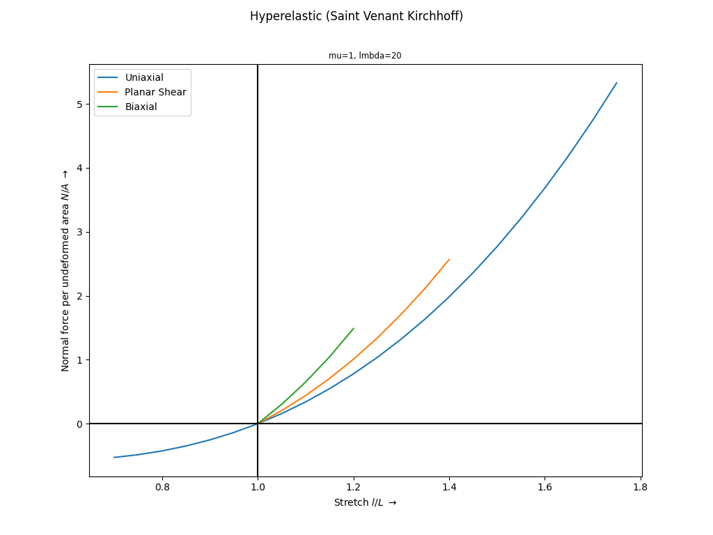
felupe.saint_venant_kirchhoff(C, mu, lmbda)

Strain energy function of the isotropic hyperelastic Saint-Venant Kirchhoff material formulation.

Parameters:

• C (tensortrax.Tensor) – Right Cauchy-Green deformation tensor.

• mu (float) – Second Lamé constant (shear modulus).

• lmbda (float) – First Lamé constant (shear modulus).

Notes

The strain energy function is given in Eq. (30)

(30)\[\psi = \mu I_2 + \lambda \frac{I_1^2}{2}\]

with the first and second invariant of the Green-Lagrange strain tensor \(\boldsymbol{E} = \frac{1}{2} (\boldsymbol{C} - \boldsymbol{1})\), see Eq. (31).

(31)\[ \begin{align}\begin{aligned}I_1 &= \text{tr}\left( \boldsymbol{E} \right)\\I_2 &= \boldsymbol{E} : \boldsymbol{E}\end{aligned}\end{align} \]

Examples

Warning

The Saint-Venant Kirchhoff material formulation is unstable for large strains.

>>> import felupe as fem
>>>
>>> umat = fem.Hyperelastic(fem.saint_venant_kirchhoff, mu=1.0, lmbda=20.0)
>>> ax = umat.plot(incompressible=False)

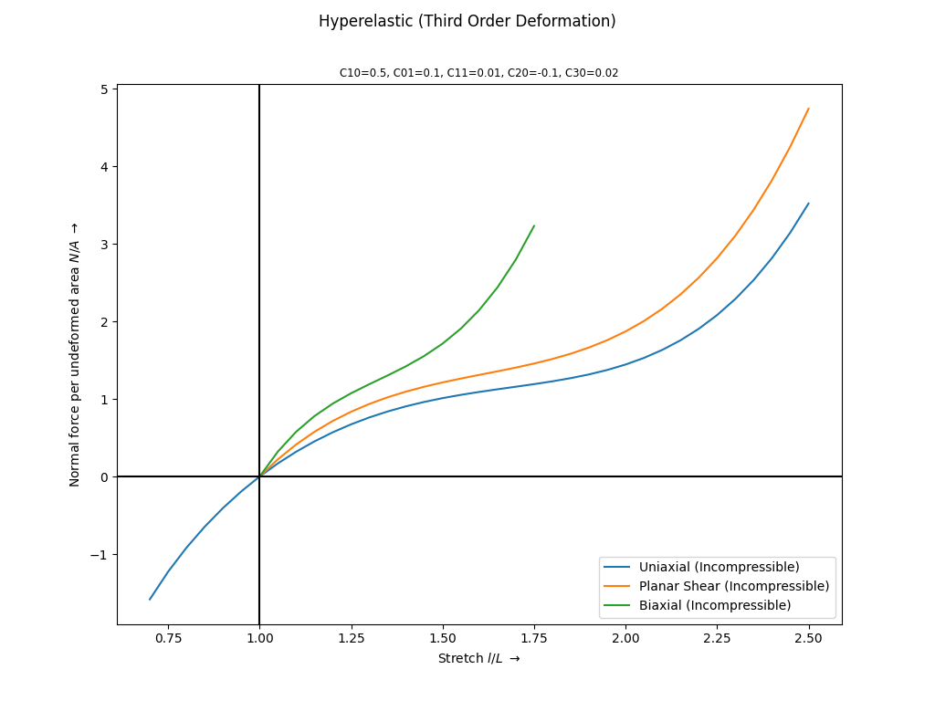
felupe.third_order_deformation(C, C10, C01, C11, C20, C30)

Strain energy function of the isotropic hyperelastic Third-Order-Deformation material formulation.

Parameters:

• C (tensortrax.Tensor) – Right Cauchy-Green deformation tensor.

• C10 (float) – Material parameter associated to the linear term of the first invariant.

• C01 (float) – Material parameter associated to the linear term of the second invariant.

• C11 (float) – Material parameter associated to the mixed term of the first and second invariant.

• C20 (float) – Material parameter associated to the quadratic term of the first invariant.

• C30 (float) – Material parameter associated to the cubic term of the first invariant.

Notes

The strain energy function is given in Eq. (32)

(32)\[ \begin{align}\begin{aligned}\psi &= C_{10} \left(\hat{I}_1 - 3 \right) + C_{01} \left(\hat{I}_2 - 3 \right) + C_{11} \left(\hat{I}_1 - 3 \right) \left(\hat{I}_2 - 3 \right)\\ &+ C_{20} \left(\hat{I}_1 - 3 \right)^2 + C_{30} \left(\hat{I}_1 - 3 \right)^3\end{aligned}\end{align} \]

with the first and second main invariant of the distortional part of the right Cauchy-Green deformation tensor, see Eq. (33).

(33)\[ \begin{align}\begin{aligned}\hat{I}_1 &= J^{-2/3} \text{tr}\left( \boldsymbol{C} \right)\\\hat{I}_2 &= J^{-4/3} \frac{1}{2} \left( \text{tr}\left(\boldsymbol{C}\right)^2 - \text{tr}\left(\boldsymbol{C}^2\right) \right)\end{aligned}\end{align} \]

The doubled sum of the material parameters \(C_{10}\) and \(C_{01}\) is equal to the initial shear modulus \(\mu\) as denoted in Eq. (34).

(34)\[\mu = 2 \left( C_{10} + C_{01} \right)\]

Examples

>>> import felupe as fem
>>>
>>> umat = fem.Hyperelastic(
...     fem.third_order_deformation, C10=0.5, C01=0.1, C11=0.01, C20=-0.1, C30=0.02
... )
>>> ax = umat.plot(incompressible=True)

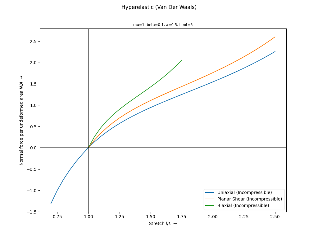
felupe.van_der_waals(C, mu, limit, a, beta)

Strain energy function of the Van der Waals [1]_ material formulation.,

Parameters:

• C (tensortrax.Tensor) – Right Cauchy-Green deformation tensor.

• mu (float) – Initial shear modulus.

• limit (float) – Limiting stretch \(\lambda_m\) at which the polymer chain network becomes locked.

• a (float) – Attractive interactions between the quasi-particles.

• beta (float) – Mixed-Invariant factor: 0 for pure I1- and 1 for pure I2-contribution.

Examples

>>> import felupe as fem
>>>
>>> umat = fem.Hyperelastic(fem.van_der_waals, mu=1.0, beta=0.1, a=0.5, limit=5.0)
>>> ax = umat.plot(incompressible=True)

References

[1]

H.-G. Kilian, “Equation of state of real networks”, Polymer, vol. 22, no. 2. Elsevier BV, pp. 209–217, Feb. 1981. doi: 10.1016/0032-3861(81)90200-7.

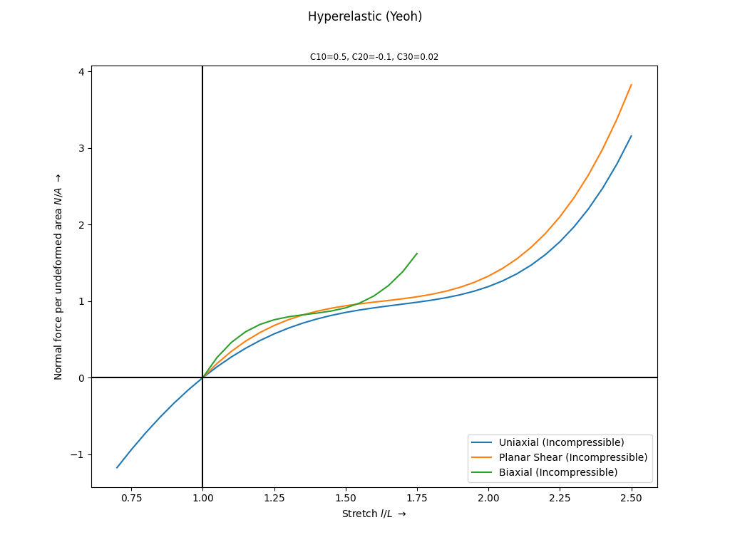
felupe.yeoh(C, C10, C20, C30)

Strain energy function of the isotropic hyperelastic Yeoh material formulation.

Parameters:

• C (tensortrax.Tensor) – Right Cauchy-Green deformation tensor.

• C10 (float) – Material parameter associated to the linear term of the first invariant.

• C20 (float) – Material parameter associated to the quadratic term of the first invariant.

• C30 (float) – Material parameter associated to the cubic term of the first invariant.

Notes

The strain energy function is given in Eq. (35)

(35)\[\psi = C_{10} \left(\hat{I}_1 - 3 \right) + C_{20} \left(\hat{I}_1 - 3 \right)^2 + C_{30} \left(\hat{I}_1 - 3 \right)^3\]

with the first main invariant of the distortional part of the right Cauchy-Green deformation tensor, see Eq. (36).

(36)\[\hat{I}_1 = J^{-2/3} \text{tr}\left( \boldsymbol{C} \right)\]

The \(C_{10}\) material parameter is equal to half the initial shear modulus \(\mu\) as denoted in Eq. (37).

(37)\[\mu = 2 C_{10}\]

Examples

>>> import felupe as fem
>>>
>>> umat = fem.Hyperelastic(fem.yeoh, C10=0.5, C20=-0.1, C30=0.02)
>>> ax = umat.plot(incompressible=True)