Total- & Updated-Lagrange

This page contains Total- and Updated-Lagrange material formulations with automatic differentiation using tensortrax.math. The material model formulations are defined by the first Piola-Kirchhoff stress tensor. Function-decorators are available to use Total-Lagrange and Updated-Lagrange material formulations in MaterialAD.

Differentiable Tensors based on NumPy Arrays.

Frameworks

MaterialAD(fun[, nstatevars, parallel])	A material definition with a given function for the partial derivative of the strain energy function w.r.t.
total_lagrange(material)	Decorate a second Piola-Kirchhoff stress Total-Lagrange material formulation as a first Piola-Kirchoff stress function.
updated_lagrange(material)	Decorate a Cauchy-stress Updated-Lagrange material formulation as a first Piola- Kirchoff stress function.

Material Models for MaterialAD

morph(F, statevars, p)	Second Piola-Kirchhoff stress tensor of the MORPH model formulation [1]_.
morph_representative_directions(F, ...)	First Piola-Kirchhoff stress tensor of the MORPH model formulation [1]_, implemented by the concept of representative directions [2], [3].

Detailed API Reference

class felupe.MaterialAD(fun, nstatevars=0, parallel=False, **kwargs)

A material definition with a given function for the partial derivative of the strain energy function w.r.t. the deformation gradient tensor with Automatic Differentiation provided by tensortrax.

Parameters:

• fun (callable) – A gradient of the strain energy density function w.r.t. the deformation gradient tensor \(\boldsymbol{F}\). Function signature must be fun = lambda F, **kwargs: P for functions without state variables and fun = lambda F, statevars, **kwargs: [P, statevars_new] for functions with state variables. The deformation gradient tensor will be a tensortrax.Tensor when the function is evaluated. It is important to only use differentiable math-functions from tensortrax.math!

• nstatevars (int, optional) – Number of state variables (default is 0).

• parallel (bool, optional) – A flag to invoke threaded gradient of strain energy density function evaluations (default is False). May introduce additional overhead for small-sized problems.

• **kwargs (dict, optional) – Optional keyword-arguments for the gradient of the strain energy density function.

Notes

The gradient of the strain energy density function \(\frac{\partial \psi}{\partial \boldsymbol{F}}\) must be given in terms of the deformation gradient tensor \(\boldsymbol{F}\).

Warning

It is important to only use differentiable math-functions from tensortrax.math!

\[\boldsymbol{P} = \frac{\partial \psi(\boldsymbol{F}, \boldsymbol{\zeta})}{ \partial \boldsymbol{F}}\]

Take this code-block as template

import tensortrax.math as tm

def neo_hooke(F, mu):
    "First Piola-Kirchhoff stress of the Neo-Hookean material formulation."

    C = tm.dot(tm.transpose(F), F)
    Cu = tm.linalg.det(C) ** (-1/3) * C

    return mu * F @ tm.special.dev(Cu) @ tm.linalg.inv(C)

umat = fem.MaterialAD(neo_hooke, mu=1)

and this code-block for material formulations with state variables:

import tensortrax.math as tm

def viscoelastic(F, Cin, mu, eta, dtime):
    "Finite strain viscoelastic material formulation."

    # unimodular part of the right Cauchy-Green deformation tensor
    C = tm.dot(tm.transpose(F), F)
    Cu = tm.linalg.det(C) ** (-1 / 3) * C

    # update of state variables by evolution equation
    Ci = tm.special.from_triu_1d(Cin, like=C) + mu / eta * dtime * Cu
    Ci = tm.linalg.det(Ci) ** (-1 / 3) * Ci

    # second Piola-Kirchhoff stress tensor
    S = mu * tm.special.dev(Cu @ tm.linalg.inv(Ci)) @ tm.linalg.inv(C)

    # first Piola-Kirchhoff stress tensor and state variable
    return F @ S, tm.special.triu_1d(Ci)

umat = fem.MaterialAD(
    viscoelastic, mu=1, eta=1, dtime=1, nstatevars=6
)

Note

See the documentation of tensortrax for further details.

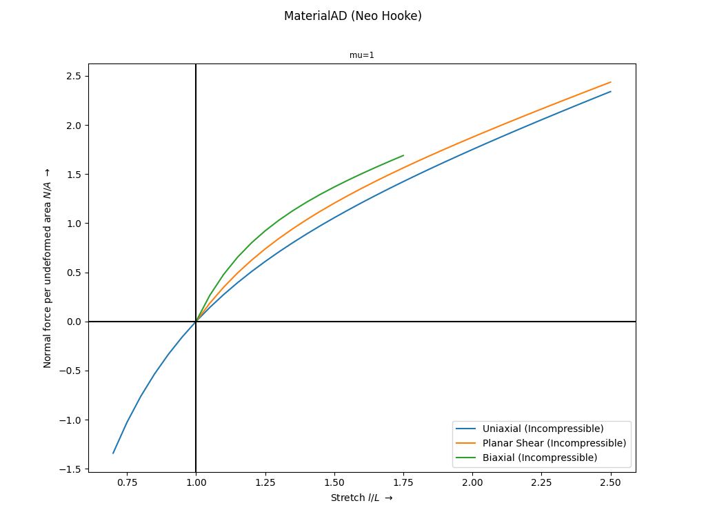
Examples

>>> import felupe as fem
>>> import tensortrax.math as tm
>>>
>>> def neo_hooke(F, mu):
...     C = tm.dot(tm.transpose(F), F)
...     S = mu * tm.special.dev(tm.linalg.det(C)**(-1/3) * C) @ tm.linalg.inv(C)
...     return F @ S
>>>
>>> umat = fem.MaterialAD(neo_hooke, mu=1)
>>> ax = umat.plot(incompressible=True)

copy()

Return a deep-copy of the constitutive material.

gradient(x)

Return the evaluated gradient of the strain energy density function.

Parameters:

x (list of ndarray) – The list with input arguments. These contain the extracted fields of a FieldContainer along with the old vector of state variables, [*field.extract(), statevars_old].

Returns:

A list with the evaluated gradient(s) of the strain energy density function and the updated vector of state variables.

Return type:

list of ndarray

hessian(x)

Return the evaluated upper-triangle components of the hessian(s) of the strain energy density function.

Parameters:

x (list of ndarray) – The list with input arguments. These contain the extracted fields of a FieldContainer along with the old vector of state variables, [*field.extract(), statevars_old].

Returns:

A list with the evaluated upper-triangle components of the hessian(s) of the strain energy density function.

Return type:

list of ndarray

optimize(ux=None, ps=None, bx=None, incompressible=False, relative=False, **kwargs)

Optimize the material parameters by a least-squares fit on experimental stretch-stress data.

Parameters:

• ux (array of shape (2, ...) or None, optional) – Experimental uniaxial stretch and force-per-undeformed-area data (default is None).

• ps (array of shape (2, ...) or None, optional) – Experimental planar-shear stretch and force-per-undeformed-area data (default is None).

• bx (array of shape (2, ...) or None, optional) – Experimental biaxial stretch and force-per-undeformed-area data (default is None).

• incompressible (bool, optional) – A flag to enforce incompressible deformations (default is False).

• relative (bool, optional) – A flag to optimize relative instead of absolute residuals, i.e. (predicted - observed) / observed instead of predicted - observed (default is False).

• **kwargs (dict, optional) – Optional keyword arguments are passed to scipy.optimize.least_squares().

Returns:

• ConstitutiveMaterial – A copy of the constitutive material with the optimized material parameters.

• scipy.optimize.OptimizeResult – Represents the optimization result.

Notes

Warning

At least one load case, i.e. one of the arguments ux, ps or bx must not be None.

The vector of residuals is given in Eq. (3) in case of absolute residuals

(1)\[ \begin{align}\begin{aligned}\begin{split}\boldsymbol{r} &= \begin{bmatrix} \boldsymbol{r}_\text{ux} \\ \boldsymbol{r}_\text{ps} \\ \boldsymbol{r}_\text{bx} \end{bmatrix}\end{split}\\r_\text{ux}(\lambda_i) &= P_\text{ux}(\lambda_i) - P_\text{ux, observed}(\lambda_i)\\r_\text{ps}(\lambda_i) &= P_\text{ps}(\lambda_i) - P_\text{ps, observed}(\lambda_i)\\r_\text{bx}(\lambda_i) &= P_\text{bx}(\lambda_i) - P_\text{bx, observed}(\lambda_i)\end{aligned}\end{align} \]

and in Eq. (4) in case of relative residuals.

(2)\[ \begin{align}\begin{aligned}\begin{split}\boldsymbol{r} &= \begin{bmatrix} \boldsymbol{r}_\text{ux} \\ \boldsymbol{r}_\text{ps} \\ \boldsymbol{r}_\text{bx} \end{bmatrix}\end{split}\\r_\text{ux}(\lambda_i) &= \frac{ P_\text{ux}(\lambda_i) - P_\text{ux, observed}(\lambda_i)}{ P_\text{ux, observed}(\lambda_i) }\\r_\text{ps}(\lambda_i) &= \frac{ P_\text{ps}(\lambda_i) - P_\text{ps, observed}(\lambda_i)}{ P_\text{ps, observed}(\lambda_i) }\\r_\text{bx}(\lambda_i) &= \frac{ P_\text{bx}(\lambda_i) - P_\text{bx, observed}(\lambda_i)}{ P_\text{bx, observed}(\lambda_i) }\end{aligned}\end{align} \]

Examples

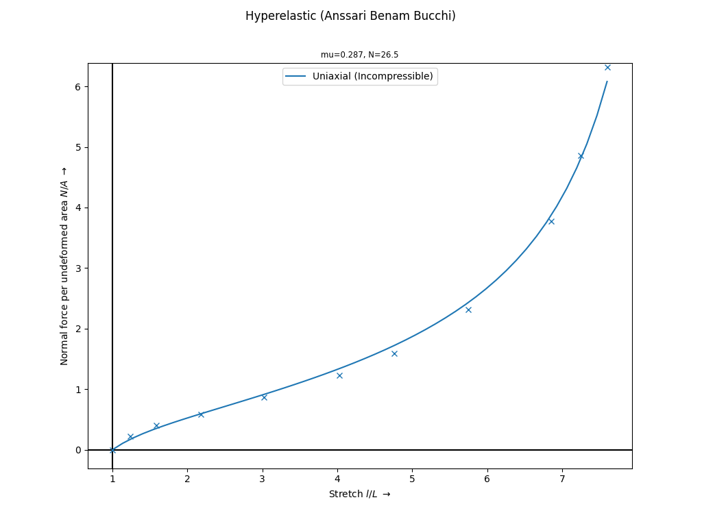
The Anssari-Benam Bucchi material model formulation is best-fitted on Treloar’s uniaxial and biaxial tension data [1]_.

>>> import numpy as np
>>> import felupe as fem
>>>
>>> λ, P = np.array(
...     [
...         [1.000, 0.00],
...         [1.240, 2.30],
...         [1.585, 4.16],
...         [2.180, 6.00],
...         [3.020, 8.80],
...         [4.030, 12.5],
...         [4.760, 16.2],
...         [5.750, 23.6],
...         [6.850, 38.5],
...         [7.250, 49.6],
...         [7.600, 64.4],
...     ]
... ).T * np.array([[1.0], [0.0980665]])
>>>
>>> umat = fem.Hyperelastic(fem.anssari_benam_bucchi)
>>> umat_new, res = umat.optimize(
...     ux=[λ, P], incompressible=True, relative=True
... )
>>>
>>> ux = np.linspace(λ.min(), λ.max(), num=50)
>>> ax = umat_new.plot(incompressible=True, ux=ux, bx=None, ps=None)

>>> ax.plot(λ, P, "C0x")

See also

scipy.optimize.least_squares

Solve a nonlinear least-squares problem with bounds on the variables.

References

[1]

L. R. G. Treloar, “Stress-strain data for vulcanised rubber under various types of deformation”, Transactions of the Faraday Society, vol. 40. Royal Society of Chemistry (RSC), p. 59, 1944. doi: 10.1039/tf9444000059. Data available at https://www.uni-due.de/mathematik/ag_neff/neff_hencky.

plot(incompressible=False, **kwargs)

Return a plot with normal force per undeformed area vs. stretch curves for the elementary homogeneous deformations uniaxial tension/compression, planar shear and biaxial tension of a given isotropic material formulation.

Parameters:

• incompressible (bool, optional) – A flag to enforce views on incompressible deformations (default is False).

• **kwargs (dict, optional) – Optional keyword-arguments for ViewMaterial or ViewMaterialIncompressible.

Return type:

matplotlib.axes.Axes

See also

felupe.ViewMaterial

Create views on normal force per undeformed area vs. stretch curves for the elementary homogeneous deformations uniaxial tension/compression, planar shear and biaxial tension of a given isotropic material formulation.

felupe.ViewMaterialIncompressible

Create views on normal force per undeformed area vs. stretch curves for the elementary homogeneous incompressible deformations uniaxial tension/compression, planar shear and biaxial tension of a given isotropic material formulation.

screenshot(filename='umat.png', incompressible=False, **kwargs)

Save a screenshot with normal force per undeformed area vs. stretch curves for the elementary homogeneous deformations uniaxial tension/compression, planar shear and biaxial tension of a given isotropic material formulation.

Parameters:

• filename (str, optional) – The filename of the screenshot (default is “umat.png”).

• incompressible (bool, optional) – A flag to enforce views on incompressible deformations (default is False).

• **kwargs (dict, optional) – Optional keyword-arguments for ViewMaterial or ViewMaterialIncompressible.

Return type:

matplotlib.axes.Axes

See also

felupe.ViewMaterial

Create views on normal force per undeformed area vs. stretch curves for the elementary homogeneous deformations uniaxial tension/compression, planar shear and biaxial tension of a given isotropic material formulation.

felupe.ViewMaterialIncompressible

Create views on normal force per undeformed area vs. stretch curves for the elementary homogeneous incompressible deformations uniaxial tension/compression, planar shear and biaxial tension of a given isotropic material formulation.

view(incompressible=False, **kwargs)

Create views on normal force per undeformed area vs. stretch curves for the elementary homogeneous deformations uniaxial tension/compression, planar shear and biaxial tension of a given isotropic material formulation.

Parameters:

• incompressible (bool, optional) – A flag to enforce views on incompressible deformations (default is False).

• **kwargs (dict, optional) – Optional keyword-arguments for ViewMaterial or ViewMaterialIncompressible.

Return type:

felupe.ViewMaterial or felupe.ViewMaterialIncompressible

See also

felupe.ViewMaterial

Create views on normal force per undeformed area vs. stretch curves for the elementary homogeneous deformations uniaxial tension/compression, planar shear and biaxial tension of a given isotropic material formulation.

felupe.ViewMaterialIncompressible

Create views on normal force per undeformed area vs. stretch curves for the elementary homogeneous incompressible deformations uniaxial tension/compression, planar shear and biaxial tension of a given isotropic material formulation.

felupe.morph(F, statevars, p)

Second Piola-Kirchhoff stress tensor of the MORPH model formulation [1]_.

Parameters:

• C (tensortrax.Tensor) – Right Cauchy-Green deformation tensor.

• statevars (array) – Vector of stacked state variables (CTS, C, SA).

• p (list of float) – A list which contains the 8 material parameters.

Notes

The MORPH material model is implemented as a second Piola-Kirchhoff stress-based formulation with automatic differentiation. The Tresca invariant of the distortional part of the right Cauchy-Green deformation tensor is used as internal state variable, see Eq. (3).

Warning

While the MORPH-material formulation captures the Mullins effect and quasi-static hysteresis effects of rubber mixtures very nicely, it has been observed to be unstable for medium- to highly-distorted states of deformation.

(3)\[ \begin{align}\begin{aligned}\boldsymbol{C} &= \boldsymbol{F}^T \boldsymbol{F}\\I_3 &= \det (\boldsymbol{C})\\\hat{\boldsymbol{C}} &= I_3^{-1/3} \boldsymbol{C}\\\hat{\lambda}^2_\alpha &= \text{eigvals}(\hat{\boldsymbol{C}})\\\hat{C}_T &= \max \left( \hat{\lambda}^2_\alpha - \hat{\lambda}^2_\beta \right)\\\hat{C}_T^S &= \max \left( \hat{C}_T, \hat{C}_{T,n}^S \right)\end{aligned}\end{align} \]

A sigmoid-function is used inside the deformation-dependent variables \(\alpha\), \(\beta\) and \(\gamma\), see Eq. (4).

(4)\[ \begin{align}\begin{aligned}f(x) &= \frac{1}{\sqrt{1 + x^2}}\\\alpha &= p_1 + p_2 \ f(p_3\ C_T^S)\\\beta &= p_4\ f(p_3\ C_T^S)\\\gamma &= p_5\ C_T^S\ \left( 1 - f\left(\frac{C_T^S}{p_6}\right) \right)\end{aligned}\end{align} \]

The rate of deformation is described by the Lagrangian tensor and its Tresca- invariant, see Eq. (5).

Note

It is important to evaluate the incremental right Cauchy-Green tensor by the difference of the final and the previous state of deformation, not by its variation with respect to the deformation gradient tensor.

(5)\[ \begin{align}\begin{aligned}\hat{\boldsymbol{L}} &= \text{sym}\left( \text{dev}(\boldsymbol{C}^{-1} \Delta\boldsymbol{C}) \right) \hat{\boldsymbol{C}}\\\lambda_{\hat{\boldsymbol{L}}, \alpha} &= \text{eigvals}(\hat{\boldsymbol{L}})\\\hat{L}_T &= \max \left( \lambda_{\hat{\boldsymbol{L}}, \alpha}-\lambda_{\hat{\boldsymbol{L}}, \beta} \right)\\\Delta\boldsymbol{C} &= \boldsymbol{C} - \boldsymbol{C}_n\end{aligned}\end{align} \]

The additional stresses evolve between the limiting stresses, see Eq. (6). The additional deviatoric-enforcement terms [1]_ are neglected in this implementation.

(6)\[ \begin{align}\begin{aligned}\boldsymbol{S}_L &= \left( \gamma \exp \left(p_7 \frac{\hat{\boldsymbol{L}}}{\hat{L}_T} \frac{\hat{C}_T}{\hat{C}_T^S} \right) + p8 \frac{\hat{\boldsymbol{L}}}{\hat{L}_T} \right) \boldsymbol{C}^{-1}\\\boldsymbol{S}_A &= \frac{ \boldsymbol{S}_{A,n} + \beta\ \hat{L}_T\ \boldsymbol{S}_L }{1 + \beta\ \hat{L}_T}\\\boldsymbol{S} &= 2 \alpha\ \text{dev}( \hat{\boldsymbol{C}} ) \boldsymbol{C}^{-1}+\text{dev}\left(\boldsymbol{S}_A\ \boldsymbol{C}\right) \boldsymbol{C}^{-1}\end{aligned}\end{align} \]

Note

Only the upper-triangle entries of the symmetric stress-tensor state variables are stored in the solid body. Hence, it is necessary to extract such variables with tm.special.from_triu_1d() and export them as tm.special.triu_1d().

Examples

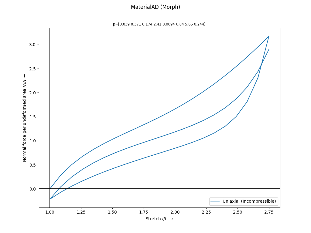
>>> import felupe as fem
>>>
>>> umat = fem.MaterialAD(
...     fem.morph,
...     p=[0.039, 0.371, 0.174, 2.41, 0.0094, 6.84, 5.65, 0.244],
...     nstatevars=13,
... )
>>> ax = umat.plot(
...    incompressible=True,
...    ux=fem.math.linsteps(
...        # [1, 2, 1, 2.75, 1, 3.5, 1, 4.2, 1, 4.8, 1, 4.8, 1],
...        [1, 2.75, 1, 2.75],
...        num=20,
...    ),
...    ps=None,
...    bx=None,
... )

References

[1]

D. Besdo and J. Ihlemann, “A phenomenological constitutive model for rubberlike materials and its numerical applications”, International Journal of Plasticity, vol. 19, no. 7. Elsevier BV, pp. 1019–1036, Jul. 2003. doi: 10.1016/s0749-6419(02)00091-8.

See also

felupe.morph_representative_directions

Strain energy function of the MORPH model formulation, implemented by the concept of representative directions.

felupe.morph_representative_directions(F, statevars, p, ε=1e-08)

First Piola-Kirchhoff stress tensor of the MORPH model formulation [1]_, implemented by the concept of representative directions [2], [3].

Parameters:

• C (tensortrax.Tensor) – Right Cauchy-Green deformation tensor.

• statevars (array) – Vector of stacked state variables (CTS, λ - 1, SA1, SA2).

• p (list of float) – A list which contains the 8 material parameters.

• ε (float, optional) – A small stabilization parameter (default is 1e-8).

Examples

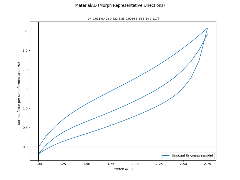
>>> import felupe as fem
>>>
>>> umat = fem.MaterialAD(
...     fem.morph_representative_directions,
...     p=[0.011, 0.408, 0.421, 6.85, 0.0056, 5.54, 5.84, 0.117],
...     nstatevars=84,
... )
>>> ax = umat.plot(
...    incompressible=True,
...    ux=fem.math.linsteps(
...        # [1, 2, 1, 2.75, 1, 3.5, 1, 4.2, 1, 4.8, 1, 4.8, 1],
...        [1, 2.75, 1, 2.75],
...        num=20,
...    ),
...    ps=None,
...    bx=None,
... )

References

[1]

D. Besdo and J. Ihlemann, “A phenomenological constitutive model for rubberlike materials and its numerical applications”, International Journal of Plasticity, vol. 19, no. 7. Elsevier BV, pp. 1019–1036, Jul. 2003. doi: 10.1016/s0749-6419(02)00091-8.

[2] (1,2)

M. Freund, “Verallgemeinerung eindimensionaler Materialmodelle für die Finite-Elemente-Methode”, Dissertation, Technische Universität Chemnitz, Chemnitz, 2013.

[3] (1,2)

C. Miehe, S. Göktepe and F. Lulei, “A micro-macro approach to rubber-like materials - Part I: the non-affine micro-sphere model of rubber elasticity”, Journal of the Mechanics and Physics of Solids, vol. 52, no. 11. Elsevier BV, pp. 2617–2660, Nov. 2004. doi: 10.1016/j.jmps.2004.03.011.

See also

felupe.morph

Strain energy function of the MORPH model formulation.

felupe.total_lagrange(material)

Decorate a second Piola-Kirchhoff stress Total-Lagrange material formulation as a first Piola-Kirchoff stress function.

Notes

\[\delta \psi = \boldsymbol{F} \boldsymbol{S} : \delta \boldsymbol{F}\]

Examples

>>> import felupe as fem
>>> import tensortrax.math as tm
>>>
>>> @fem.total_lagrange
>>> def neo_hooke_total_lagrange(F, mu=1):
>>>     C = F.T @ F
>>>     S = mu * tm.special.dev(tm.linalg.det(C)**(-1/3) * C) @ tm.linalg.inv(C)
>>>     return S
>>>
>>> umat = fem.MaterialAD(neo_hooke_total_lagrange, mu=1)

See also

felupe.Hyperelastic

A hyperelastic material definition with a given function for the strain energy density function per unit undeformed volume with Automatic Differentiation.

felupe.MaterialAD

A material definition with a given function for the partial derivative of the strain energy function w.r.t. the deformation gradient tensor with Automatic Differentiation.

felupe.updated_lagrange(material)

Decorate a Cauchy-stress Updated-Lagrange material formulation as a first Piola- Kirchoff stress function.

Notes

\[\delta \psi = J \boldsymbol{\sigma} \boldsymbol{F}^{-T} : \delta \boldsymbol{F}\]

Examples

>>> import felupe as fem
>>> import tensortrax.math as tm
>>>
>>> @fem.updated_lagrange
>>> def neo_hooke_updated_lagrange(F, mu=1):
>>>     J = tm.linalg.det(F)
>>>     b = F @ F.T
>>>     σ = mu * tm.special.dev(J**(-2/3) * b) / J
>>>     return σ
>>>
>>> umat = fem.MaterialAD(neo_hooke_updated_lagrange, mu=1)

See also

felupe.Hyperelastic

A hyperelastic material definition with a given function for the strain energy density function per unit undeformed volume with Automatic Differentiation.

felupe.MaterialAD

A material definition with a given function for the partial derivative of the strain energy function w.r.t. the deformation gradient tensor with Automatic Differentiation.