Element

This module provides classes for the finite element formulations.

Element()

Base-class for a finite element which provides methods for plotting.

Linear Elements

Vertex()	A vertex element formulation with constant shape functions.
Line()	A 1D line element formulation with linear shape functions.
Quad()	A 2D quadrilateral element formulation with linear shape functions.
Hexahedron()	A 3D hexahedron (brick) element formulation with linear shape functions.
Triangle()	A 2D triangle element formulation with linear shape functions.
Tetra()	A 3D tetrahedron element formulation with linear shape functions.

Constant Elements

ConstantQuad()	A 2D quadrilateral element formulation with constant shape functions.
ConstantHexahedron()	A 3D hexahedron (brick) element formulation with constant shape functions.

Quadratic Elements

QuadraticQuad()	A 2D quadrilateral element formulation with quadratic (serendipity) shape functions.
QuadraticHexahedron()	A 3D hexahedron (brick) element formulation with quadratic (serendipity) shape functions.
BiQuadraticQuad()	A 2D quadrilateral element formulation with bi-quadratic shape functions.
TriQuadraticHexahedron()	A 3D hexahedron (brick) element formulation with tri-quadratic shape functions.
QuadraticTriangle()	A 2D triangle element formulation with quadratic shape functions.
QuadraticTetra()	A 3D tetrahedron element formulation with quadratic shape functions.

Bubble-Enriched Elements

TriangleMINI([bubble_multiplier])	A 2D triangle element formulation with bubble-enriched linear shape functions.
TetraMINI([bubble_multiplier])	A 3D tetrahedron element formulation with bubble-enriched linear shape functions.

Arbitrary-Order Elements

element.ArbitraryOrderLagrange(order, dim[, ...])

A n-dimensional Lagrange finite element (e.g. line, quad or hexahdron) of arbitrary order.

Detailed API Reference

class felupe.Element

Bases: object

Base-class for a finite element which provides methods for plotting.

Examples

This example shows how to implement a hexahedron element.

>>> import felupe as fem
>>> import numpy as np
>>>
>>> class Hexahedron(fem.Element):
...     def __init__(self):
...         a = [-1, 1, 1, -1, -1, 1, 1, -1]
...         b = [-1, -1, 1, 1, -1, -1, 1, 1]
...         c = [-1, -1, -1, -1, 1, 1, 1, 1]
...         self.points = np.vstack([a, b, c]).T
...
...         # additional attributes for plotting, optional
...         self.cells = np.array([[0, 1, 2, 3, 4, 5, 6, 7]])
...         self.cell_type = "hexahedron"
...
...     def function(self, rst):
...         r, s, t = rst
...         a, b, c = self.points.T
...         ar, bs, ct = 1 + a * r, 1 + b * s, 1 + c * t
...         return (ar * bs * ct) / 8
...
...     def gradient(self, rst):
...         r, s, t = rst
...         a, b, c = self.points.T
...         ar, bs, ct = 1 + a * r, 1 + b * s, 1 + c * t
...         return np.stack([a * bs * ct, ar * b * ct, ar * bs * c], axis=1)
>>>
>>> mesh = fem.Cube(n=6)
>>> element = Hexahedron()
>>> quadrature = fem.GaussLegendre(order=1, dim=3)
>>> region = fem.Region(mesh, element, quadrature)

The gradient (and optionally the hessian) may be carried out using automatic differentiation.

Warning

It is important to use only differentiable math-functions from tensortrax.math!

>>> import felupe as fem
>>> import tensortrax as tr
>>> import numpy as np
>>>
>>> class Hexahedron(fem.Element):
...     def __init__(self):
...         a = [-1, 1, 1, -1, -1, 1, 1, -1]
...         b = [-1, -1, 1, 1, -1, -1, 1, 1]
...         c = [-1, -1, -1, -1, 1, 1, 1, 1]
...         self.points = np.vstack([a, b, c]).T
...
...         # additional attributes for plotting, optional
...         self.cells = np.array([[0, 1, 2, 3, 4, 5, 6, 7]])
...         self.cell_type = "hexahedron"
...
...     def fun(self, rst):
...         a, b, c = tr.math.array(self.points.T, shape=(3, 8), like=rst)
...         r, s, t = rst
...         ar, bs, ct = 1 + a * r, 1 + b * s, 1 + c * t
...         return (ar * bs * ct) / 8
...
...     def function(self, rst):
...         return tr.function(self.fun)(rst)
...
...     def gradient(self, rst):
...         return tr.jacobian(self.fun)(rst)
...
...     def hessian(self, rst):
...         return tr.hessian(self.fun)(rst)
>>>
>>> mesh = fem.Cube(n=6)
>>> element = Hexahedron()
>>> quadrature = fem.GaussLegendre(order=1, dim=3)
>>> region = fem.Region(mesh, element, quadrature, hess=True)

plot(*args, style='wireframe', color='black', add_axes_at_origin=True, add_point_labels=True, show_points=True, font_size=26, **kwargs)

Plot the element.

See also

felupe.Scene.plot

Plot method of a scene.

screenshot(*args, filename=None, transparent_background=None, scale=None, **kwargs)

Take a screenshot of the element.

See also

pyvista.Plotter.screenshot

Take a screenshot of a PyVista plotter.

view(point_data=None, cell_data=None, cell_type=None)

View the element with optional given dicts of point- and cell-data items.

Parameters:

• point_data (dict or None, optional) – Additional point-data dict (default is None).

• cell_data (dict or None, optional) – Additional cell-data dict (default is None).

• cell_type (pyvista.CellType or None, optional) – Cell-type of PyVista (default is None).

Returns:

A object which provides visualization methods for felupe.element.Element.

Return type:

felupe.ViewMesh

See also

felupe.ViewMesh

Visualization methods for felupe.Mesh.

class felupe.Vertex

Bases: Element

A vertex element formulation with constant shape functions.

Notes

The vertex element is defined by one point.

function(r)

Return the shape functions at given coordinate (r).

gradient(r)

Return the gradient of shape functions at given coordinate (r).

hessian(rs)

Return the hessian of shape functions at given coordinate (r).

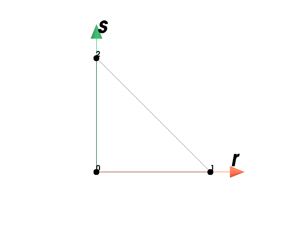
class felupe.Line

Bases: Element

A 1D line element formulation with linear shape functions.

Notes

The linear line element is defined by two points (0-1). [1]

The shape functions \(\boldsymbol{h}\) are given in terms of the coordinates \((r)\).

\[\begin{split}\boldsymbol{h}(r) = \frac{1}{2} \begin{bmatrix} (1-r) \\ (1+r) \end{bmatrix}\end{split}\]

References

[1]

W. Schroeder, K. Martin and B. Lorensen. The Visualization Toolkit, 4th ed. Kitware, 2006. ISBN: 978-1-930934-19-1.

function(rv)

Return the shape functions at given coordinates (r,).

gradient(rv)

Return the gradient of shape functions at given coordinates (r,).

hessian(rv)

Return the hessian of shape functions at given coordinates (r,).

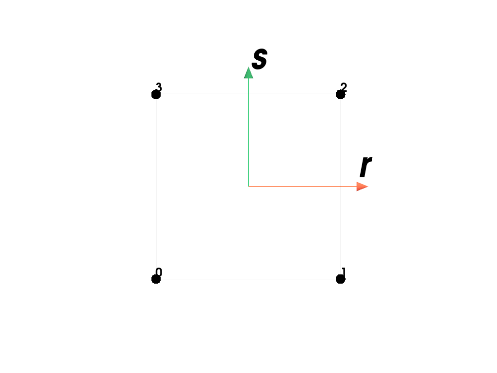
class felupe.Quad

Bases: Element

A 2D quadrilateral element formulation with linear shape functions.

Notes

The quadrilateral element is defined by four points (0-3). [1]

The shape functions \(\boldsymbol{h}\) are given in terms of the coordinates \((r,s)\).

\[\begin{split}\boldsymbol{h}(r,s) = \frac{1}{4} \begin{bmatrix} (1-r) (1-s) \\ (1+r) (1-s) \\ (1+r) (1+s) \\ (1-r) (1+s) \end{bmatrix}\end{split}\]

Examples

>>> import felupe as fem
>>>
>>> element = fem.Quad()
>>> element.plot().show()

References

[1]

W. Schroeder, K. Martin and B. Lorensen. The Visualization Toolkit, 4th ed. Kitware, 2006. ISBN: 978-1-930934-19-1.

function(rs)

Return the shape functions at given coordinates (r, s).

gradient(rs)

Return the gradient of shape functions at given coordinates (r, s).

hessian(rs)

Return the hessian of shape functions at given coordinates (r, s).

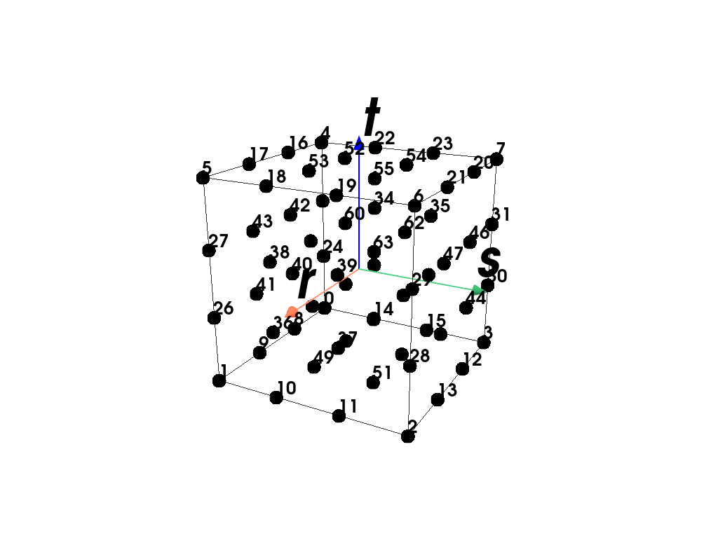
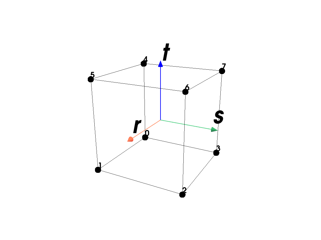
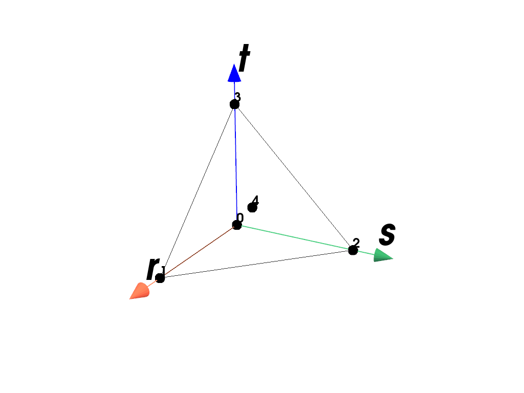
class felupe.Hexahedron

Bases: Element

A 3D hexahedron (brick) element formulation with linear shape functions.

Notes

The hexahedron element is defined by eight points (0-7) where (0,1,2,3) forms the base and (4,5,6,7) the opposite quad. [1]

The shape functions \(\boldsymbol{h}\) are given in terms of the coordinates \((r,s,t)\).

\[\begin{split}\boldsymbol{h}(r,s,t) = \frac{1}{8} \begin{bmatrix} (1-r) (1-s) (1-t) \\ (1+r) (1-s) (1-t) \\ (1+r) (1+s) (1-t) \\ (1-r) (1+s) (1-t) \\ (1-r) (1-s) (1+t) \\ (1+r) (1-s) (1+t) \\ (1+r) (1+s) (1+t) \\ (1-r) (1+s) (1+t) \end{bmatrix}\end{split}\]

Examples

>>> import felupe as fem
>>>
>>> element = fem.Hexahedron()
>>> element.plot().show()

References

[1]

W. Schroeder, K. Martin and B. Lorensen. The Visualization Toolkit, 4th ed. Kitware, 2006. ISBN: 978-1-930934-19-1.

function(rst)

Return the shape functions at given coordinates (r, s, t).

gradient(rst)

Return the gradient of shape functions at given coordinates (r, s, t).

hessian(rst)

Return the hessian of shape functions at given coordinates (r, s, t).

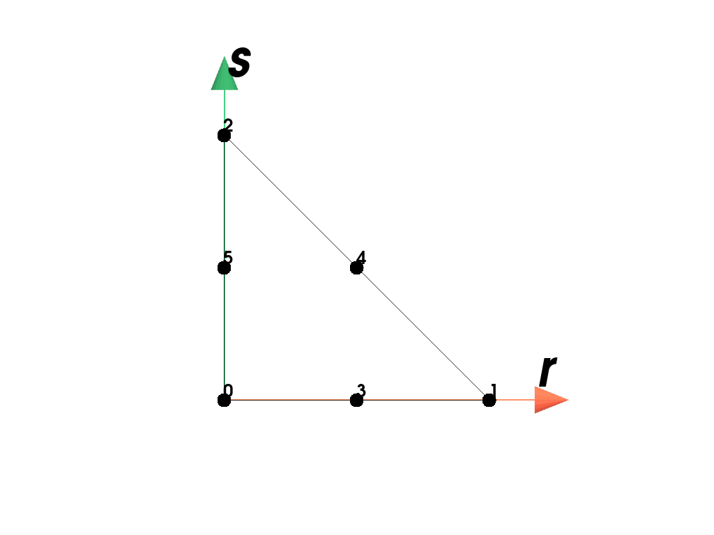
class felupe.Triangle

Bases: Element

A 2D triangle element formulation with linear shape functions.

Notes

The triangle element is defined by three points (0-2). [1]

The shape functions \(\boldsymbol{h}\) are given in terms of the coordinates \((r,s)\) [2]_.

\[\begin{split}\boldsymbol{h}(r,s) = \begin{bmatrix} 1-r-s \\ r \\ s \end{bmatrix}\end{split}\]

Examples

>>> import felupe as fem
>>>
>>> element = fem.Triangle()
>>> element.plot().show()

References

[1]

W. Schroeder, K. Martin and B. Lorensen. The Visualization Toolkit, 4th ed. Kitware, 2006. ISBN: 978-1-930934-19-1.

[2]

K. J. Bathe, Finite element procedures, 2nd ed. K. J. Bathe, Watertown, MA, 2014.

function(rs)

Return the shape functions at given coordinates (r, s).

gradient(rs)

Return the gradient of shape functions at given coordinates (r, s).

hessian(rs)

Return the hessian of shape functions at given coordinates (r, s).

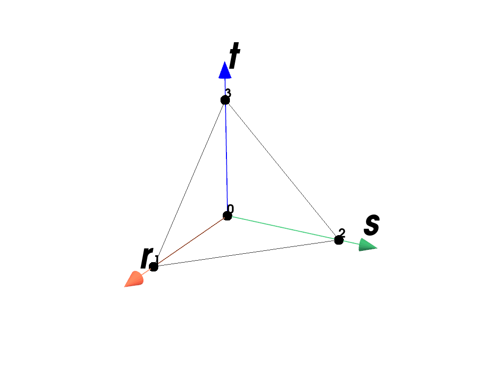
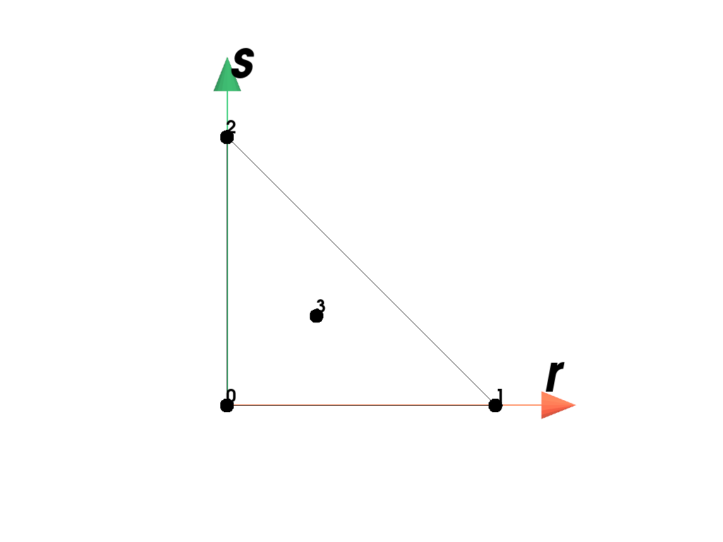
class felupe.Tetra

Bases: Element

A 3D tetrahedron element formulation with linear shape functions.

Notes

The tetrahedron element is defined by four points (0-3). [1]

The shape functions \(\boldsymbol{h}\) are given in terms of the coordinates \((r,s,t)\).

\[\begin{split}\boldsymbol{h}(r,s,t) = \begin{bmatrix} 1-r-s-t \\ r \\ s \\ t \end{bmatrix}\end{split}\]

Examples

>>> import felupe as fem
>>>
>>> element = fem.Tetra()
>>> element.plot().show()

References

[1]

W. Schroeder, K. Martin and B. Lorensen. The Visualization Toolkit, 4th ed. Kitware, 2006. ISBN: 978-1-930934-19-1.

function(rst)

Return the shape functions at given coordinates (r, s, t).

gradient(rst)

Return the gradient of shape functions at given coordinates (r, s, t).

hessian(rst)

Return the hessian of shape functions at given coordinates (r, s, t).

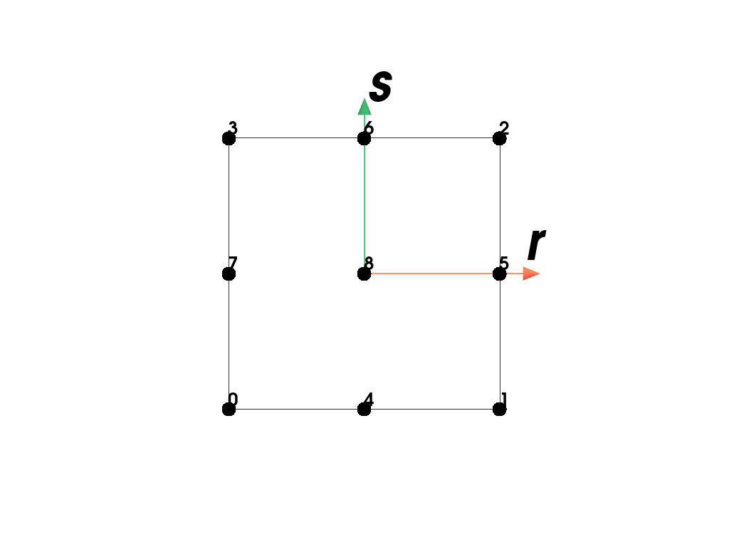
class felupe.ConstantQuad

Bases: Element

A 2D quadrilateral element formulation with constant shape functions.

Notes

The quadrilateral element is defined by four points (0-3). [1]

The shape function \(h\) is given in terms of the coordinates \((r,s)\).

\[h(r,s) = 1\]

Examples

>>> import felupe as fem
>>>
>>> element = fem.ConstantQuad()
>>> element.plot().show()

References

[1]

W. Schroeder, K. Martin and B. Lorensen. The Visualization Toolkit, 4th ed. Kitware, 2006. ISBN: 978-1-930934-19-1.

function(rs)

Return the shape functions at given coordinates (r, s).

gradient(rs)

Return the gradient of shape functions at given coordinates (r, s).

hessian(rs)

Return the hessian of shape functions at given coordinates (r, s).

class felupe.ConstantHexahedron

Bases: Element

A 3D hexahedron (brick) element formulation with constant shape functions.

Notes

The hexahedron element is defined by eight points (0-7) where (0,1,2,3) forms the base and (4,5,6,7) the opposite quad. [1]

The shape function \(h\) in terms of the coordinates \((r,s,t)\) is constant and hence, its gradient is zero.

\[h(r,s,t) = 1\]

Examples

>>> import felupe as fem
>>>
>>> element = fem.ConstantHexahedron()
>>> element.plot().show()

References

[1]

W. Schroeder, K. Martin and B. Lorensen. The Visualization Toolkit, 4th ed. Kitware, 2006. ISBN: 978-1-930934-19-1.

function(rst)

Return the shape functions at given coordinates (r, s, t).

gradient(rst)

Return the gradient of shape functions at given coordinates (r, s, t).

hessian(rst)

Return the hessian of shape functions at given coordinates (r, s, t).

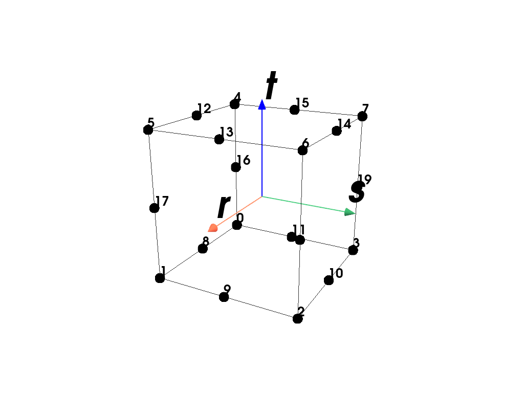
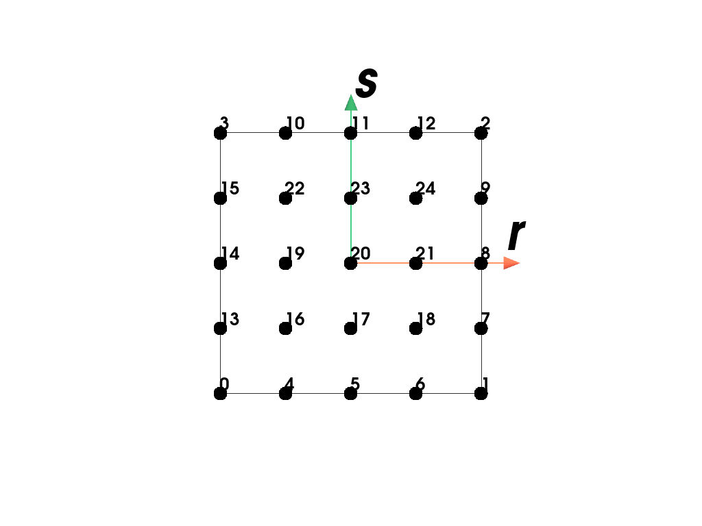
class felupe.QuadraticHexahedron

Bases: Element

A 3D hexahedron (brick) element formulation with quadratic (serendipity) shape functions.

Notes

The hexahedron element is defined by twenty points with eight corner points (0-7) where (0,1,2,3) forms the base and (4,5,6,7) the opposite quad; followed by 12 mid- edge points. The mid-edge points correspond to the edges defined by the lines between the points (0,1), (1,2), (2,3), (3,0), (4,5), (5,6), (6,7), (7,4), (0,4), (1,5), (2,6), (3,7). [1]

The shape functions \(\boldsymbol{h}\) are given in terms of the coordinates \((r,s,t)\).

Examples

>>> import felupe as fem
>>>
>>> element = fem.QuadraticHexahedron()
>>> element.plot().show()

References

[1]

W. Schroeder, K. Martin and B. Lorensen. The Visualization Toolkit, 4th ed. Kitware, 2006. ISBN: 978-1-930934-19-1.

function(rst)

Return the shape functions at given coordinates (r, s, t).

gradient(rst)

Return the gradient of shape functions at given coordinates (r, s, t).

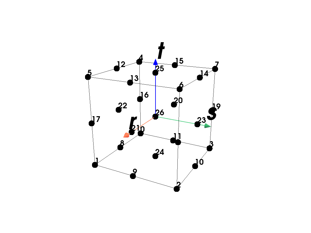
class felupe.TriQuadraticHexahedron

Bases: Element

A 3D hexahedron (brick) element formulation with tri-quadratic shape functions.

Notes

The hexahedron element is defined by 27 points. This includes 8 corner points, 12 mid-edge points, 6 mid-face points and one mid-volume point. The ordering of the 27 points defining the element is point ids (0-7,8-19, 20-25, 26) where point ids 0-7 are the eight corner vertices of the cube; followed by twelve midedge points (8-19); followed by 6 mid-face points (20-25) and the last point (26) is the mid-volume point. Note that these mid-edge points correspond to the edges defined by (0,1), (1,2), (2,3), (3,0), (4,5), (5,6), (6,7), (7,4), (0,4), (1,5), (2,6), (3,7). The mid-surface points lie on the faces defined by (first edge point id’s, than mid-edge point id’s): (0,1,5,4;8,17,12,16), (1,2,6,5;9,18,13,17), (2,3,7,6,10,19,14,18), (3,0,4,7;11,16,15,19), (0,1,2,3;8,9,10,11), (4,5,6,7;12,13,14,15). The last point lies in the center (0,1,2,3,4,5,6,7). [1]

The shape functions \(\boldsymbol{h}\) are given in terms of the coordinates \((r,s,t)\).

Examples

>>> import felupe as fem
>>>
>>> element = fem.TriQuadraticHexahedron()
>>> element.plot().show()

References

[1]

W. Schroeder, K. Martin and B. Lorensen. The Visualization Toolkit, 4th ed. Kitware, 2006. ISBN: 978-1-930934-19-1.

function(rst)

Return the shape functions at given coordinates (r, s, t).

gradient(rst)

Return the gradient of shape functions at given coordinates (r, s, t).

hessian(rst)

Return the hessian of shape functions at given coordinates (r, s, t).

class felupe.QuadraticQuad

Bases: Element

A 2D quadrilateral element formulation with quadratic (serendipity) shape functions.

Notes

The quadratic (serendipity) quadrilateral element is defined by eight points (0-7). [1]

The shape functions \(\boldsymbol{h}\) are given in terms of the coordinates \((r,s)\).

Examples

>>> import felupe as fem
>>>
>>> element = fem.QuadraticQuad()
>>> element.plot().show()

References

[1]

W. Schroeder, K. Martin and B. Lorensen. The Visualization Toolkit, 4th ed. Kitware, 2006. ISBN: 978-1-930934-19-1.

function(rs)

Return the shape functions at given coordinates (r, s).

gradient(rs)

Return the gradient of shape functions at given coordinates (r, s).

hessian(rs)

Return the hessian of shape functions at given coordinates (r, s).

class felupe.BiQuadraticQuad

Bases: Element

A 2D quadrilateral element formulation with bi-quadratic shape functions.

Notes

The bi-quadratic quadrilateral element is defined by nine points (0-8). [1]

The shape functions \(\boldsymbol{h}\) are given in terms of the coordinates \((r,s)\).

Examples

>>> import felupe as fem
>>>
>>> element = fem.BiQuadraticQuad()
>>> element.plot().show()

References

[1]

W. Schroeder, K. Martin and B. Lorensen. The Visualization Toolkit, 4th ed. Kitware, 2006. ISBN: 978-1-930934-19-1.

function(rs)

Return the shape functions at given coordinates (r, s).

gradient(rs)

Return the gradient of shape functions at given coordinates (r, s).

hessian(rs)

Return the hessian of shape functions at given coordinates (r, s).

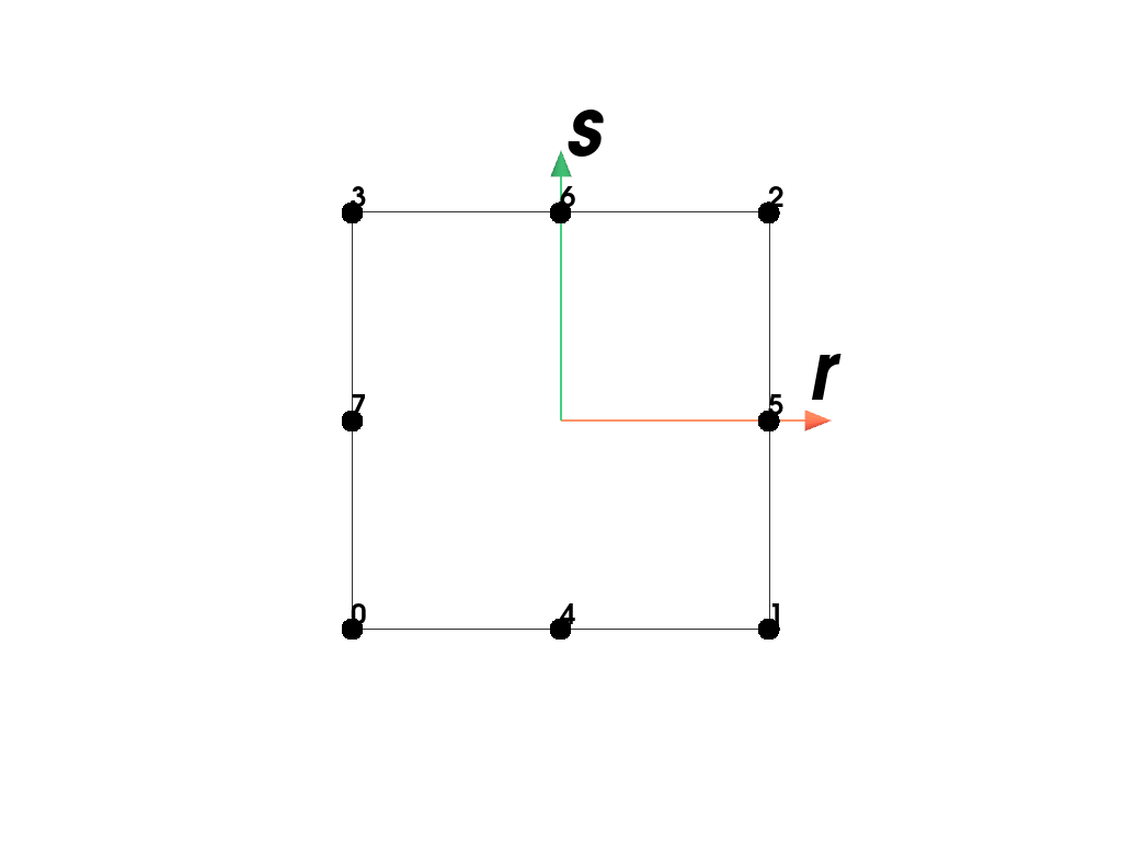
class felupe.QuadraticTriangle

Bases: Element

A 2D triangle element formulation with quadratic shape functions.

Notes

The quadratic triangle element is defined by six points (0-5). The element includes three mid-edge points besides the three triangle vertices. The ordering of the three points defining the element is point ids (0-2,3-5) where id #3 is the mid-edge point between points (0,1); id #4 is the mid-edge point between points (1,2); and id #5 is the mid-edge point between points (2,0). [1]

The shape functions \(\boldsymbol{h}\) are given in terms of the coordinates \((r,s)\) [2]_.

\[\begin{split}\boldsymbol{h}(r,s) = \begin{bmatrix} 1-r-s \\ r \\ s \\ 4 r (1-r-s) \\ 4 r s \\ 4 s (1-r-s) \end{bmatrix}\end{split}\]

Examples

>>> import felupe as fem
>>>
>>> element = fem.QuadraticTriangle()
>>> element.plot().show()

References

[1]

W. Schroeder, K. Martin and B. Lorensen. The Visualization Toolkit, 4th ed. Kitware, 2006. ISBN: 978-1-930934-19-1.

[2]

K. J. Bathe, Finite element procedures, 2nd ed. K. J. Bathe, Watertown, MA, 2014.

function(rs)

Return the shape functions at given coordinates (r, s).

gradient(rs)

Return the gradient of shape functions at given coordinates (r, s).

class felupe.QuadraticTetra

Bases: Element

A 3D tetrahedron element formulation with quadratic shape functions.

Notes

The quadratic tetrahedron element is defined by ten points (0-9). The element includes a mid-edge point on each of the edges of the tetrahedron. The ordering of the ten points defining the cell is point ids (0-3,4-9) where ids 0-3 are the four tetra vertices; and point ids 4-9 are the mid-edge points between (0,1), (1,2), (2,0), (0,3), (1,3), and (2,3). [1]

The shape functions \(\boldsymbol{h}\) are given in terms of the coordinates \((r,s,t)\).

\[\begin{split}\boldsymbol{h}(r,s,t) = \begin{bmatrix} t_1 (2 t_1 - 1) \\ t_2 (2 t_2 - 1) \\ t_3 (2 t_3 - 1) \\ t_4 (2 t_4 - 1) \\ 4 t_1 t_2 \\ 4 t_2 t_3 \\ 4 t_3 t_1 \\ 4 t_1 t_4 \\ 4 t_2 t_4 \\ 4 t_3 t_4 \end{bmatrix}\end{split}\]

with

\[ \begin{align}\begin{aligned}t_1 &= 1 - r - s - t\\t_2 &= r\\t_3 &= s\\t_4 &= t\end{aligned}\end{align} \]

Examples

>>> import felupe as fem
>>>
>>> element = fem.QuadraticTetra()
>>> element.plot().show()

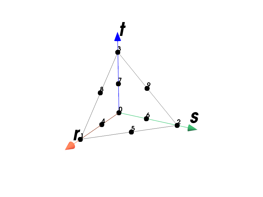
References

[1]

W. Schroeder, K. Martin and B. Lorensen. The Visualization Toolkit, 4th ed. Kitware, 2006. ISBN: 978-1-930934-19-1.

function(rst)

Return the shape functions at given coordinates (r, s, t).

gradient(rst)

Return the gradient of shape functions at given coordinates (r, s, t).

class felupe.TriangleMINI(bubble_multiplier=1.0)

Bases: Element

A 2D triangle element formulation with bubble-enriched linear shape functions.

Notes

The MINI triangle element is defined by four points (0-3). [1]

The shape functions \(\boldsymbol{h}\) are given in terms of the coordinates \((r,s)\).

\[\begin{split}\boldsymbol{h}(r,s) = \begin{bmatrix} 1-r-s \\ r \\ s \\ r s (1-r-s) \end{bmatrix}\end{split}\]

Examples

>>> import felupe as fem
>>>
>>> element = fem.TriangleMINI()
>>> element.plot().show()

References

[1]

W. Schroeder, K. Martin and B. Lorensen. The Visualization Toolkit, 4th ed. Kitware, 2006. ISBN: 978-1-930934-19-1.

function(rs)

Return the shape functions at given coordinates (r, s).

gradient(rs)

Return the gradient of shape functions at given coordinates (r, s).

hessian(rs)

Return the hessian of shape functions at given coordinates (r, s).

class felupe.TetraMINI(bubble_multiplier=1.0)

Bases: Element

A 3D tetrahedron element formulation with bubble-enriched linear shape functions.

Notes

The MINI tetrahedron element is defined by five points (0-4). [1]

The shape functions \(\boldsymbol{h}\) are given in terms of the coordinates \((r,s,t)\).

\[\begin{split}\boldsymbol{h}(r,s,t) = \begin{bmatrix} 1-r-s-t \\ r \\ s \\ t \\ r s t (1-r-s-t) \end{bmatrix}\end{split}\]

Examples

>>> import felupe as fem
>>>
>>> element = fem.TetraMINI()
>>> element.plot().show()

References

[1]

W. Schroeder, K. Martin and B. Lorensen. The Visualization Toolkit, 4th ed. Kitware, 2006. ISBN: 978-1-930934-19-1.

function(rst)

Return the shape functions at given coordinates (r, s, t).

gradient(rst)

Return the gradient of shape functions at given coordinates (r, s, t).

hessian(rst)

Return the hessian of shape functions at given coordinates (r, s, t).

class felupe.element.ArbitraryOrderLagrange(order, dim, interval=(-1, 1), permute=True)

Bases: Element

A n-dimensional Lagrange finite element (e.g. line, quad or hexahdron) of arbitrary order.

Notes

Polynomial shape functions

The basis function vector is generated with row-stacking of the individual lagrange polynomials. Each polynomial defined in the interval \([-1,1]\) is a function of the parameter \(r\). The curve parameters matrix \(\boldsymbol{A}\) is of symmetric shape due to the fact that for each evaluation point \(r_j\) exactly one basis function \(h_j(r)\) is needed.

\[\boldsymbol{h}(r) = \boldsymbol{A}^T \boldsymbol{r}(r)\]

Curve parameter matrix

The evaluation of the curve parameter matrix \(\boldsymbol{A}\) is carried out by boundary conditions. Each shape function \(h_i\) has to take the value of one at the associated nodal coordinate \(r_i\) and zero at all other point coordinates.

\[ \begin{align}\begin{aligned}\boldsymbol{A}^T \boldsymbol{R} &= \boldsymbol{I} \qquad \text{with} \qquad \boldsymbol{R} = \begin{bmatrix}\boldsymbol{r}(r_1) & \boldsymbol{r}(r_2) & \dots & \boldsymbol{r}(r_p)\end{bmatrix}\\\boldsymbol{A}^T &= \boldsymbol{R}^{-1}\end{aligned}\end{align} \]

Interpolation and partial derivatives

The approximation of nodal unknowns \(\hat{\boldsymbol{u}}\) as a function of the parameter \(r\) is evaluated as

\[\boldsymbol{u}(r) \approx \hat{\boldsymbol{u}}^T \boldsymbol{h}(r)\]

For the calculation of the partial derivative of the interpolation field w.r.t. the parameter \(r\) a simple shift of the entries of the parameter vector is enough. This shifted parameter vector is denoted as \(\boldsymbol{r}^-\). A minus superscript indices the negative shift of the vector entries by \(-1\).

\[ \begin{align}\begin{aligned}\frac{\partial \boldsymbol{u}(r)}{\partial r} &\approx \hat{\boldsymbol{u}}^T \frac{\partial \boldsymbol{h}(r)}{\partial r}\\\frac{\partial \boldsymbol{h}(r)}{\partial r} &= \boldsymbol{A}^T \boldsymbol{r}^-(r) \qquad \text{with} \qquad r_0^- = 0 \qquad \text{and} \qquad r_i^- = \frac{r^{(i-1)}}{(i-1)!} \qquad \text{for} \qquad i=(1 \dots p)\end{aligned}\end{align} \]

n-dimensional shape functions

Multi-dimensional shape function matrices \(\boldsymbol{H}_{2D}, \boldsymbol{H}_{3D}\) are simply evaluated as dyadic (outer) vector products of one-dimensional shape function vectors. The multi- dimensional shape function vector is a one-dimensional representation (flattened version) of the multi-dimensional shape function matrix.

\[ \begin{align}\begin{aligned}\boldsymbol{H}_{2D}(r,s) &= \boldsymbol{h}(r) \otimes \boldsymbol{h}(s)\\\boldsymbol{H}_{3D}(r,s,t) &= \boldsymbol{h}(r) \otimes \boldsymbol{h}(s) \otimes \boldsymbol{h}(t)\end{aligned}\end{align} \]

Examples

>>> import felupe as fem
>>>
>>> element = fem.ArbitraryOrderLagrangeElement(order=4, dim=2)
>>> element.plot().show()

>>> import felupe as fem
>>>
>>> element = fem.ArbitraryOrderLagrangeElement(order=3, dim=3)
>>> element.plot().show()

function(r)

Return the shape functions at given coordinate vector r.

gradient(r)

Return the gradient of shape functions at given coordinate vector r.

hessian(r)

Return the hessian of shape functions at given coordinate vector r.