Note
Go to the end to download the full example code.
Elastic bearing with torsional loading#
This example requires external packages.
pip install pypardiso
An elastic bearing is subjected to combined multiaxial radial-torsional-cardanic loading. First the meshes for the rubber and the metal sheet rings are created.
import numpy as np
import pypardiso

import felupe as fem

# inner and outer line meshes for the rubber
bottom = fem.mesh.Line(a=-50, b=50, n=6)
top = fem.mesh.Line(a=-30, b=30, n=6)

# embed line meshes in 2d-space
bottom.update(np.pad(bottom.points, ((0, 0), (0, 1)), constant_values=30))
top.update(np.pad(top.points, ((0, 0), (0, 1)), constant_values=60))

# fill face with quads between the two line meshes, add realistic runouts
section = fem.mesh.fill_between(bottom, top, n=8)
section = section.add_runouts(axis=1, centerpoint=[0, 45], values=[0.2], normalize=True)

# revolve the face for the rubber volume
rubber = section.revolve(n=19, phi=360)

# create meshes for the metal sheet rings
metal = fem.MeshContainer(
    [
        fem.Rectangle(a=(-50, 25), b=(50, 30), n=(6, 3)).revolve(n=19, phi=360),
        fem.Rectangle(a=(-30, 60), b=(30, 65), n=(6, 3)).revolve(n=19, phi=360),
    ],
    merge=True,
).stack()
Sub-regions are generated for all materials. The same applies to the material formulations as well as the solid bodies. The sub-fields are also created as vector- valued displacement fields. However, the fields must be merged in a top-level field- container. This modifies the sub-fields to be used in the solid bodies.
regions = [fem.RegionHexahedron(m) for m in [rubber, metal]]
fields, field = fem.FieldContainer([fem.Field(r, dim=3) for r in regions]).merge()

# material formulations and solid bodies for the rubber and the metal sheets
umats = [fem.NeoHooke(mu=1), fem.LinearElasticLargeStrain(E=2.1e5, nu=0.3)]
solids = [
    fem.SolidBodyNearlyIncompressible(umats[0], fields[0], bulk=5000),
    fem.SolidBody(umats[1], fields[1]),
]
The boundary conditions are created on the top-level displacement field. Masks are created for both the innermost and the outermost metal sheet faces. The global field holds a mesh-container attribute which may be used for plotting.
x, y, z = field.region.mesh.points.T

boundaries = fem.BoundaryDict(
    inner=fem.dof.Boundary(field[0], mask=np.isclose(np.sqrt(y**2 + z**2), 25)),
    outer=fem.dof.Boundary(field[0], mask=np.isclose(np.sqrt(y**2 + z**2), 65)),
)

boundaries.plot(
    plotter=field.mesh_container.plot(colors=[[0.3, 0.3, 0.3], "white"], opacity=1.0)
).show()

# prescribed values for the innermost radial mesh points
table = fem.math.linsteps([0, 1], num=3)
move = []

for progress in table:
    inner = field.region.mesh.points[boundaries["inner"].points]
    inner_rotated = fem.math.rotate_points(
        points=inner,
        angle_deg=30 * progress,
        axis=0,
        center=[0, 0, 0],
    )
    inner_rotated = fem.math.rotate_points(
        points=inner_rotated,
        angle_deg=-5 * progress,
        axis=1,
        center=[0, 0, 0],
    )
    inner_radial = 8 * np.array([0, 0, 1]) * progress
    move.append(inner_radial + inner_rotated - inner)

After defining the load step, the simulation model is ready to be solved.
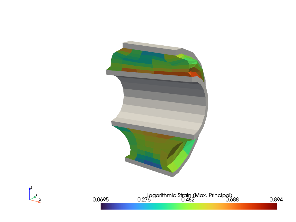
The maximum principal values of the logarithmic strain are plotted on the total simulation model as well as on a clipped view.
plotter = fields[1].plot(color="white", show_undeformed=False)
fields[0].plot(
    "Principal Values of Logarithmic Strain", show_undeformed=False, plotter=plotter
).show()

plotter = fields[1].plot(color="white", show_undeformed=False, show_edges=False)
plotter.mesh.clip("y", invert=False, value=0.0, inplace=True)

plotter = fields[0].plot(
    "Principal Values of Logarithmic Strain",
    show_undeformed=False,
    show_edges=False,
    plotter=plotter,
)
plotter.mesh.clip("y", invert=False, value=0.0, inplace=True)
plotter.show()

Total running time of the script: (0 minutes 3.112 seconds)