Note
Go to the end to download the full example code.
Nonlinear Truss Analysis#
This example requires external packages.
pip install contique
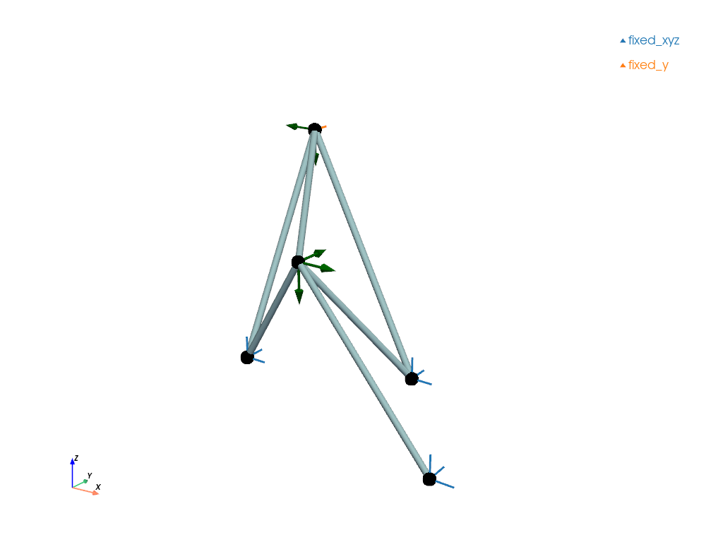
This example describes a three-dimensional system of trusses with 5 points and 6 cells (in total 5 active degrees of freedom). Given to its geometry, strong geometric nonlinearities are to be expected when the given reference load is applied. First, we create a mesh, where points are defined by their coordinates and cells by pairs of point connectivities.
import contique
import matplotlib.pyplot as plt
import numpy as np

import felupe as fem

mesh = fem.Mesh(
    points=[
        [2.5, 0, 0],
        [-1.25, 1.25, 0],
        [1, 2, 0],
        [-0.5, 1.5, 1.5],
        [-2.5, 4.5, 2.5],
    ],
    cells=[[0, 3], [1, 3], [2, 3], [2, 4], [1, 4], [3, 4]],
    cell_type="line",
)
region = fem.RegionTruss(mesh)
field = fem.FieldContainer([fem.Field(region, dim=3)])
Beside points and cells we have to define displacement boundary conditions, external forces and the constitutive material formulation for the trusses.
boundaries = fem.BoundaryDict(
    fixed_xyz=fem.Boundary(field[0], mask=[1, 1, 1, 0, 0]),
    fixed_y=fem.Boundary(field[0], mask=[0, 0, 0, 0, 1], skip=(1, 0, 1)),
)
dof0, dof1 = fem.dof.partition(field, boundaries)

solid = fem.TrussBody(
    umat=fem.LinearElastic1D(E=1),
    field=field,
    area=[0.75, 1, 0.5, 0.75, 1, 1],
)

force_3 = np.array([1, 1, -1])
force_4 = np.array([-2, 0, -2])

load_3 = fem.PointLoad(field, [3], force_3)
load_4 = fem.PointLoad(field, [4], force_4)
The undeformed configuration is plotted in a 3d-view.
plotter = mesh.plot(
    line_width=10,
    render_lines_as_tubes=True,
    show_edges=False,
)
plotter.add_points(
    mesh.points,
    color="black",
    point_size=20,
    render_points_as_spheres=True,
)
plotter = boundaries.plot(plotter=plotter)
plotter = load_3.plot(plotter=plotter, color="green", deformed=False)
plotter = load_4.plot(plotter=plotter, color="green", deformed=False)

plotter.show()
For the numeric continuation, the equilibrium function fun and its derivatives
w.r.t. the displacement field dfun_du and the load-proportionality-factor
dfun_dlpf have to be defined. Here, we’re only interested in the active degrees of
freedom.
def fun(x, lpf, *args):
    field[0].values.ravel()[dof1] = x
    load_3.update(force_3 * lpf)
    load_4.update(force_4 * lpf)
    return fem.tools.fun([solid, load_3, load_4], field)[dof1]


def dfun_du(x, lpf, *args):
    field[0].values.ravel()[dof1] = x
    K = fem.tools.jac([solid, load_3, load_4], field)
    return fem.solve.partition(field, K, dof1, dof0)[2]


def dfun_dlpf(x, lpf, *args):
    load_3.update(force_3)
    load_4.update(force_4)
    return fem.tools.fun([load_3, load_4], field)[dof1]
Now that the model is finished, some additional settings have to be chosen. Initial
allowed incremental system vector components for both the displacement vector and the
load-proportionality-factor (LPF) have to be specified. We use dlpf = 0.005 and
du = 0.05 (figured out after some trial and error). Both parameters can’t be
specified automatically, as they depend on the model configuration. The job will be
limited to a total amount of 163 increments (again, the total number has been figured
out after some job runs to get good looking plots).
|Step,C.| Control Component | Norm (Iter.#) | Message     |
|-------|-------------------|---------------|-------------|
|   1,1 |     5+  =>     4- | 8.8e-09 ( 6#) | => re-Cycle |
|     2 |     4-  =>     3- | 1.7e-14 ( 3#) |tol.Overshoot|
|   2,1 |     3-  =>     3- | 1.6e-14 ( 3#) |             |
|   3,1 |     3-  =>     4- | 2.3e-14 ( 3#) |tol.Overshoot|
|   4,1 |     4-  =>     4- | 6.7e-14 ( 3#) |             |
|   5,1 |     4-  =>     4- | 4.2e-13 ( 3#) |             |
|   6,1 |     4-  =>     4- | 2.5e-12 ( 3#) |             |
|   7,1 |     4-  =>     4- | 1.4e-11 ( 3#) |             |
|   8,1 |     4-  =>     4- | 7.1e-11 ( 3#) |             |
|   9,1 |     4-  =>     4- | 5.4e-11 ( 3#) |             |
|  10,1 |     4-  =>     4- | 3.8e-11 ( 3#) |             |
|  11,1 |     4-  =>     4- | 3.0e-11 ( 3#) |             |
|  12,1 |     4-  =>     4- | 2.7e-11 ( 3#) |             |
|  13,1 |     4-  =>     4- | 2.7e-11 ( 3#) |             |
|  14,1 |     4-  =>     4- | 3.1e-11 ( 3#) |             |
|  15,1 |     4-  =>     4- | 4.0e-11 ( 3#) |             |
|  16,1 |     4-  =>     4- | 5.4e-11 ( 3#) |             |
|  17,1 |     4-  =>     4- | 7.6e-11 ( 3#) |             |
|  18,1 |     4-  =>     4- | 1.1e-10 ( 3#) |             |
|  19,1 |     4-  =>     4- | 1.6e-10 ( 3#) |             |
|  20,1 |     4-  =>     4- | 2.3e-10 ( 3#) |             |
|  21,1 |     4-  =>     4- | 3.3e-10 ( 3#) |             |
|  22,1 |     4-  =>     4- | 4.6e-10 ( 3#) |             |
|  23,1 |     4-  =>     4- | 6.1e-10 ( 3#) |             |
|  24,1 |     4-  =>     4- | 6.5e-10 ( 3#) |             |
|  25,1 |     4-  =>     4- | 3.4e-10 ( 3#) |             |
|  26,1 |     4-  =>     4- | 4.1e-10 ( 3#) |             |
|  27,1 |     4-  =>     4- | 1.9e-15 ( 4#) |             |
|  28,1 |     4-  =>     4- | 2.5e-13 ( 4#) |             |
|  29,1 |     4-  =>     2- | 4.7e-11 ( 4#) |tol.Overshoot|
|  30,1 |     2-  =>     2- | 9.4e-13 ( 4#) |             |
|  31,1 |     2-  =>     2- | 1.9e-12 ( 4#) |             |
|  32,1 |     2-  =>     2- | 3.9e-09 ( 4#) |             |
|  33,1 |     2-  =>     2- | 7.3e-03 ( 8#) |Failed       |
|  34,1 |     2-  =>     4+ | 5.4e-02 ( 8#) |Failed       |
|  35,1 |     2-  =>     4+ | 4.0e-11 ( 4#) |tol.Overshoot|
|  36,1 |     4+  =>     4+ | 2.2e-09 ( 3#) |             |
|  37,1 |     4+  =>     4+ | 2.4e-10 ( 3#) |             |
|  38,1 |     4+  =>     4+ | 2.5e-10 ( 3#) |             |
|  39,1 |     4+  =>     4+ | 1.6e-10 ( 3#) |             |
|  40,1 |     4+  =>     4+ | 3.5e-11 ( 3#) |             |
|  41,1 |     4+  =>     4+ | 1.8e-10 ( 3#) |             |
|  42,1 |     4+  =>     4+ | 1.3e-09 ( 3#) |             |
|  43,1 |     4+  =>     4+ | 7.3e-10 ( 3#) |             |
|  44,1 |     4+  =>     4+ | 2.9e-10 ( 3#) |             |
|  45,1 |     4+  =>     4+ | 1.0e-10 ( 3#) |             |
|  46,1 |     4+  =>     4+ | 3.5e-11 ( 3#) |             |
|  47,1 |     4+  =>     4+ | 1.5e-11 ( 3#) |             |
|  48,1 |     4+  =>     4+ | 1.5e-11 ( 3#) |             |
|  49,1 |     4+  =>     4+ | 1.8e-11 ( 3#) |             |
|  50,1 |     4+  =>     4+ | 2.1e-11 ( 3#) |             |
|  51,1 |     4+  =>     4+ | 2.3e-11 ( 3#) |             |
|  52,1 |     4+  =>     4+ | 2.5e-11 ( 3#) |             |
|  53,1 |     4+  =>     4+ | 2.8e-11 ( 3#) |             |
|  54,1 |     4+  =>     4+ | 3.2e-11 ( 3#) |             |
|  55,1 |     4+  =>     4+ | 3.8e-11 ( 3#) |             |
|  56,1 |     4+  =>     4+ | 4.7e-11 ( 3#) |             |
|  57,1 |     4+  =>     4+ | 6.2e-11 ( 3#) |             |
|  58,1 |     4+  =>     4+ | 8.9e-11 ( 3#) |             |
|  59,1 |     4+  =>     4+ | 1.4e-10 ( 3#) |             |
|  60,1 |     4+  =>     4+ | 2.3e-10 ( 3#) |             |
|  61,1 |     4+  =>     4+ | 4.3e-10 ( 3#) |             |
|  62,1 |     4+  =>     4+ | 9.0e-10 ( 3#) |             |
|  63,1 |     4+  =>     4+ | 2.1e-09 ( 3#) |             |
|  64,1 |     4+  =>     4+ | 5.4e-09 ( 3#) |             |
|  65,1 |     4+  =>     3+ | 2.3e-15 ( 4#) |tol.Overshoot|
|  66,1 |     3+  =>     3+ | 1.9e-09 ( 3#) |             |
|  67,1 |     3+  =>     3+ | 1.5e-09 ( 3#) |             |
|  68,1 |     3+  =>     3+ | 3.4e-09 ( 3#) |             |
|  69,1 |     3+  =>     3+ | 2.4e-15 ( 4#) |             |
|  70,1 |     3+  =>     3+ | 6.5e-04 ( 8#) |Failed       |
|  71,1 |     3+  =>     3+ | 1.4e-15 ( 4#) |             |
|  72,1 |     3+  =>     3+ | 7.0e-04 ( 8#) |Failed       |
|  73,1 |     3+  =>     3+ | 3.1e-15 ( 4#) |             |
|  74,1 |     3+  =>     2- | 4.2e-03 ( 8#) |Failed       |
|  75,1 |     3+  =>     2- | 1.5e-14 ( 4#) |tol.Overshoot|
|  76,1 |     2-  =>     2- | 3.6e-11 ( 3#) |             |
|  77,1 |     2-  =>     2- | 1.2e-11 ( 3#) |             |
|  78,1 |     2-  =>     2- | 4.1e-11 ( 3#) |             |
|  79,1 |     2-  =>     2- | 1.4e-10 ( 3#) |             |
|  80,1 |     2-  =>     2- | 5.4e-10 ( 3#) |             |
|  81,1 |     2-  =>     3- | 2.5e-09 ( 3#) |tol.Overshoot|
|  82,1 |     3-  =>     3- | 4.2e-14 ( 4#) |             |
|  83,1 |     3-  =>     3- | 4.3e-15 ( 4#) |             |
|  84,1 |     3-  =>     3- | 7.9e-09 ( 3#) |             |
|  85,1 |     3-  =>     3- | 7.5e-09 ( 3#) |             |
|  86,1 |     3-  =>     3- | 3.7e-10 ( 3#) |             |
|  87,1 |     3-  =>     4- | 1.7e-09 ( 3#) |tol.Overshoot|
|  88,1 |     4-  =>     4- | 3.0e-10 ( 3#) |             |
|  89,1 |     4-  =>     4- | 3.0e-10 ( 3#) |             |
|  90,1 |     4-  =>     4- | 2.5e-10 ( 3#) |             |
|  91,1 |     4-  =>     4- | 1.9e-10 ( 3#) |             |
|  92,1 |     4-  =>     4- | 1.3e-10 ( 3#) |             |
|  93,1 |     4-  =>     4- | 9.3e-11 ( 3#) |             |
|  94,1 |     4-  =>     4- | 6.5e-11 ( 3#) |             |
|  95,1 |     4-  =>     4- | 4.8e-11 ( 3#) |             |
|  96,1 |     4-  =>     4- | 3.9e-11 ( 3#) |             |
|  97,1 |     4-  =>     4- | 3.7e-11 ( 3#) |             |
|  98,1 |     4-  =>     4- | 4.3e-11 ( 3#) |             |
|  99,1 |     4-  =>     4- | 5.9e-11 ( 3#) |             |
| 100,1 |     4-  =>     4- | 9.7e-11 ( 3#) |             |
| 101,1 |     4-  =>     4- | 1.8e-10 ( 3#) |             |
| 102,1 |     4-  =>     4- | 3.9e-10 ( 3#) |             |
| 103,1 |     4-  =>     4- | 9.8e-10 ( 3#) |             |
| 104,1 |     4-  =>     4- | 3.0e-09 ( 3#) |             |
| 105,1 |     4-  =>     4- | 9.0e-16 ( 4#) |             |
| 106,1 |     4-  =>     4- | 2.9e-13 ( 4#) |             |
| 107,1 |     4-  =>     3+ | 2.5e-11 ( 5#) | => re-Cycle |
|     2 |     3+  =>     3+ | 1.5e-10 ( 4#) |             |
| 108,1 |     3+  =>     3+ | 1.9e-10 ( 4#) |             |
| 109,1 |     3+  =>     3+ | 4.3e-12 ( 4#) |             |
| 110,1 |     3+  =>     3+ | 6.1e-15 ( 4#) |             |
| 111,1 |     3+  =>     3+ | 9.7e-09 ( 3#) |             |
| 112,1 |     3+  =>     3+ | 5.6e-09 ( 3#) |             |
| 113,1 |     3+  =>     3+ | 3.2e-09 ( 3#) |             |
| 114,1 |     3+  =>     3+ | 2.0e-09 ( 3#) |             |
| 115,1 |     3+  =>     3+ | 6.7e-09 ( 3#) |             |
| 116,1 |     3+  =>     3+ | 3.8e-15 ( 4#) |             |
| 117,1 |     3+  =>     3+ | 6.1e-15 ( 4#) |             |
| 118,1 |     3+  =>     3+ | 8.0e-09 ( 3#) |             |
| 119,1 |     3+  =>     3+ | 4.2e-10 ( 3#) |             |
| 120,1 |     3+  =>     3+ | 7.0e-10 ( 3#) |             |
| 121,1 |     3+  =>     3+ | 5.9e-10 ( 3#) |             |
| 122,1 |     3+  =>     3+ | 3.0e-10 ( 3#) |             |
| 123,1 |     3+  =>     3+ | 1.3e-10 ( 3#) |             |
| 124,1 |     3+  =>     3+ | 1.1e-10 ( 3#) |             |
| 125,1 |     3+  =>     3+ | 2.6e-10 ( 3#) |             |
| 126,1 |     3+  =>     3+ | 4.5e-10 ( 3#) |             |
| 127,1 |     3+  =>     3+ | 5.5e-10 ( 3#) |             |
| 128,1 |     3+  =>     3+ | 5.1e-10 ( 3#) |             |
| 129,1 |     3+  =>     3+ | 7.0e-10 ( 3#) |             |
| 130,1 |     3+  =>     3+ | 2.3e-09 ( 3#) |             |
| 131,1 |     3+  =>     3+ | 7.3e-09 ( 3#) |             |
| 132,1 |     3+  =>     3+ | 5.0e-15 ( 4#) |             |
| 133,1 |     3+  =>     4- | 3.1e-13 ( 4#) |tol.Overshoot|
| 134,1 |     4-  =>     4- | 3.5e-14 ( 4#) |             |
| 135,1 |     4-  =>     4- | 5.1e-09 ( 3#) |             |
| 136,1 |     4-  =>     4- | 1.9e-09 ( 3#) |             |
| 137,1 |     4-  =>     4- | 1.7e-09 ( 3#) |             |
| 138,1 |     4-  =>     4- | 1.6e-09 ( 3#) |             |
| 139,1 |     4-  =>     4- | 1.2e-09 ( 3#) |             |
| 140,1 |     4-  =>     4- | 8.9e-10 ( 3#) |             |
| 141,1 |     4-  =>     4- | 8.2e-10 ( 3#) |             |
| 142,1 |     4-  =>     4- | 1.0e-09 ( 3#) |             |
| 143,1 |     4-  =>     4- | 1.5e-09 ( 3#) |             |
| 144,1 |     4-  =>     4- | 2.8e-09 ( 3#) |             |
| 145,1 |     4-  =>     4- | 6.1e-09 ( 3#) |             |
| 146,1 |     4-  =>     3- | 6.8e-16 ( 4#) |tol.Overshoot|
| 147,1 |     3-  =>     3- | 2.3e-10 ( 3#) |             |
| 148,1 |     3-  =>     3- | 8.2e-11 ( 3#) |             |
| 149,1 |     3-  =>     3- | 3.9e-11 ( 3#) |             |
| 150,1 |     3-  =>     3- | 2.7e-11 ( 3#) |             |
| 151,1 |     3-  =>     3- | 2.3e-11 ( 3#) |             |
| 152,1 |     3-  =>     3- | 2.1e-11 ( 3#) |             |
| 153,1 |     3-  =>     3- | 2.0e-11 ( 3#) |             |
| 154,1 |     3-  =>     3- | 2.1e-11 ( 3#) |             |
| 155,1 |     3-  =>     3- | 2.3e-11 ( 3#) |             |
| 156,1 |     3-  =>     3- | 2.8e-11 ( 3#) |             |
| 157,1 |     3-  =>     3- | 3.6e-11 ( 3#) |             |
| 158,1 |     3-  =>     3- | 4.8e-11 ( 3#) |             |
| 159,1 |     3-  =>     3- | 6.7e-11 ( 3#) |             |
| 160,1 |     3-  =>     3- | 9.4e-11 ( 3#) |             |
| 161,1 |     3-  =>     3- | 1.4e-10 ( 3#) |             |
| 162,1 |     3-  =>     3- | 1.9e-10 ( 3#) |             |
| 163,1 |     3-  =>     3- | 2.5e-10 ( 3#) |             |
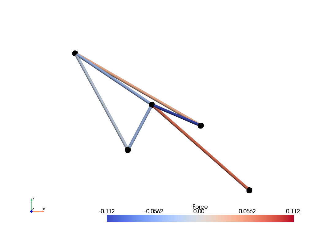
To visualize the deformed state of the model for increment 40 the deformed model plot is generated.
field[0].values.ravel()[dof1] = X[40, :-1]
force = solid.evaluate.gradient(field) * solid.area
plotter = field.view(cell_data={"Force": force}).plot(
    "Force",
    line_width=10,
    show_undeformed=False,
    view="xy",
    cmap="coolwarm",
    clim=[-abs(force).max(), abs(force).max()],
    render_lines_as_tubes=True,
    show_edges=False,
)
plotter.add_points(
    mesh.points + field[0].values,
    color="black",
    point_size=20,
    render_points_as_spheres=True,
)
plotter.show()
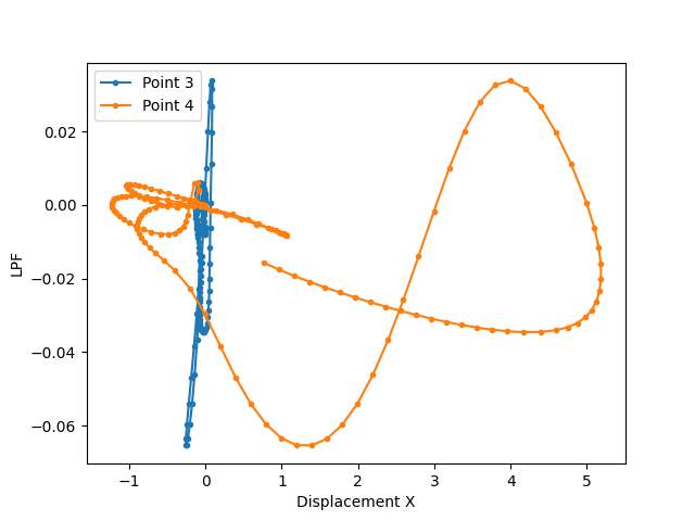
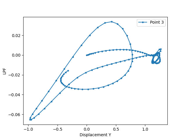
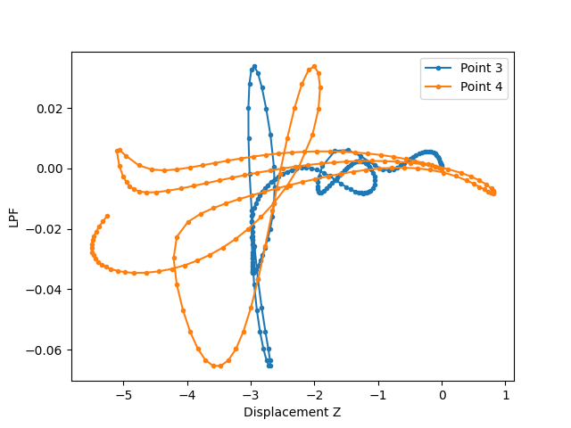
Path-tracing of the displacement-LPF curves#
The path-tracing of the deformation process is shown as a History Plot of Displacement-LPF curves for all active DOF. Strong geometrical nonlinearities are observed for all active DOF.
fig, ax = plt.subplots()
ax.plot(*X[:, [0, -1]].T, ".-", label="Point 3")
ax.plot(*X[:, [3, -1]].T, ".-", label="Point 4")
ax.set_xlabel("Displacement X")
ax.set_ylabel("LPF")
ax.legend()
fig, ax = plt.subplots()
ax.plot(*X[:, [1, -1]].T, ".-", label="Point 3")
ax.set_xlabel("Displacement Y")
ax.set_ylabel("LPF")
ax.legend()
fig, ax = plt.subplots()
ax.plot(*X[:, [2, -1]].T, ".-", label="Point 3")
ax.plot(*X[:, [4, -1]].T, ".-", label="Point 4")
ax.set_xlabel("Displacement Z")
ax.set_ylabel("LPF")
ax.legend()
Total running time of the script: (0 minutes 3.543 seconds)