Cantilever beam under gravity#
Assemble a body force vector due to gravity.
define the body force vector
linear-elastic analysis
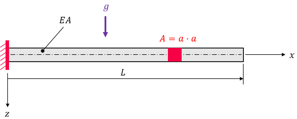
The displacement due to gravity of a cantilever beam with young’s modulus \(E=206000 N/mm^2\), poisson ratio \(\nu=0.3\), length \(L=2000 mm\) and cross section area \(A=a \cdot a\) with \(a=100 mm\) is to be evaluated within a linear-elastic analysis.
First, let’s create a meshed cube out of hexahedron cells with n=(181, 9, 9) points per axis. A numeric region created on the mesh represents the cantilever beam. A vector-valued displacement field is initiated on the region.
import numpy as np
import felupe as fe

cube = fe.Cube(a=(0, 0, 0), b=(2000, 100, 100), n=(181, 9, 9))
region = fe.RegionHexahedron(cube)
displacement = fe.Field(region, dim=3)
field = fe.FieldContainer([displacement])
A fixed boundary condition is applied on the left end of the beam. The degrees of freedom are partitioned into active (dof1) and fixed or inactive (dof0) degrees of freedom.
bounds = {"fixed": fe.dof.Boundary(displacement, fx=lambda x: x==0)}
dof0, dof1 = fe.dof.partition(field, bounds)
The material behavior is defined through a built-in isotropic linear-elastic material formulation.
umat = fe.LinearElastic(E=206000, nu=0.3)
density = 7850 * 1e-12
The body force is now assembled. Note that the gravity vector has to be reshaped for shape compatibility.
gravity = np.array([0, 0, 9.81]) * 1e3

bodyforce = fe.IntegralForm(
    fun=[density * gravity.reshape(-1, 1, 1)],
    v=field,
    dV=region.dV,
    grad_v=[False]
).assemble()
The weak form of linear elasticity is assembled into the stiffness matrix, where the constitutive elasticity matrix is generated with umat.elasticity().
stiffness = fe.IntegralForm(
    fun=umat.elasticity(region=region),
    v=field,
    dV=region.dV,
    u=field,
).assemble(parallel=True)
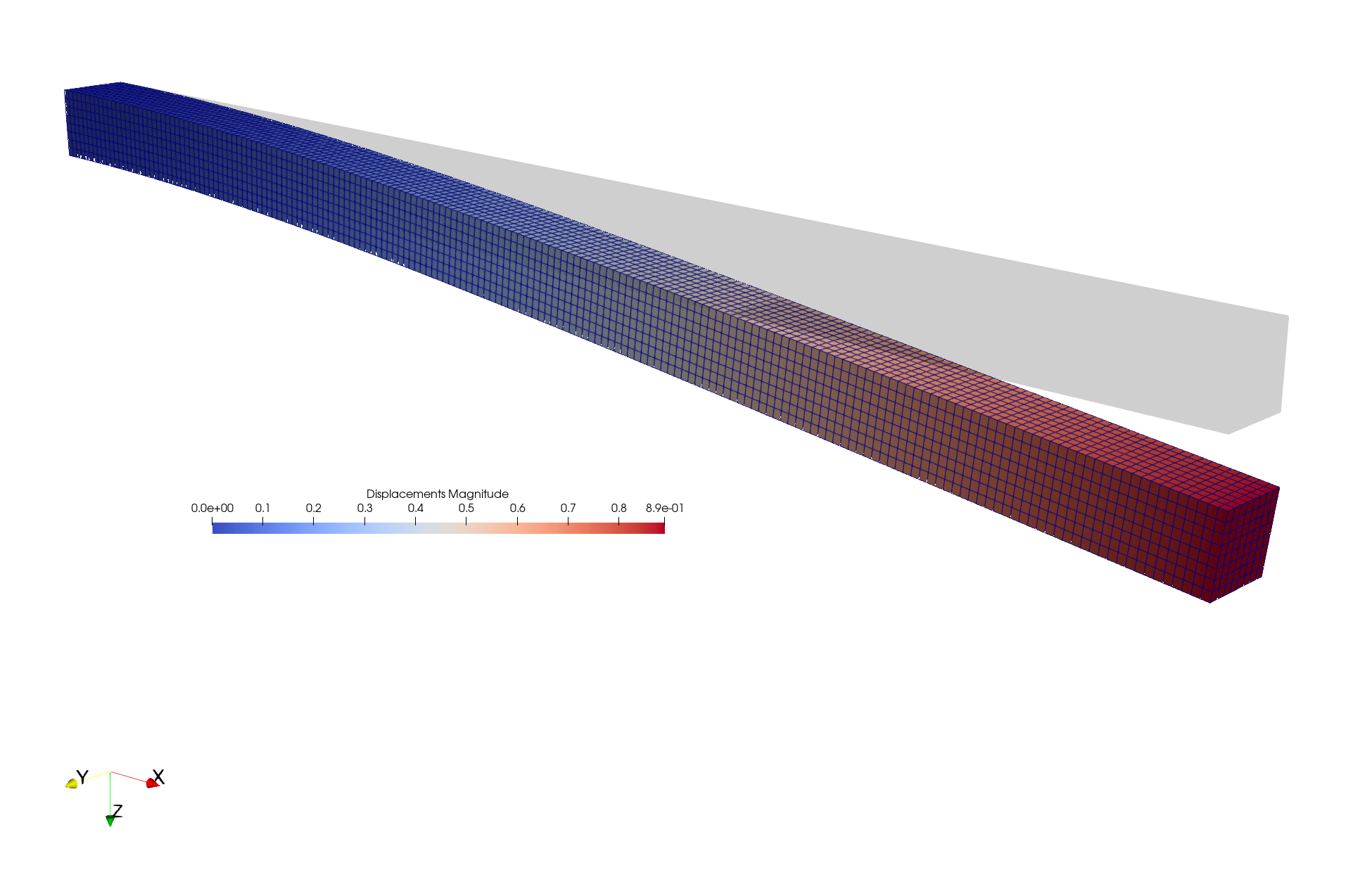
The linear equation system may now be solved. First, a partition into active and inactive degrees of freedom is performed. This partitioned system is then passed to the solver. The maximum displacement is identical to the one obtained in [1].
system = fe.solve.partition(field, stiffness, dof1, dof0, r=-bodyforce)
field += fe.solve.solve(*system)

fe.save(region, field, filename="bodyforce.vtk")
References#
[1] Glenk C. et al., Consideration of Body Forces within Finite Element Analysis, Strojniški vestnik - Journal of Mechanical Engineering, Faculty of Mechanical Engineering, 2018, ![]()