Numeric Continuation#
With the help of contique (install with pip install contique) it is possible to apply a numerical parameter continuation algorithm on any system of equilibrium equations. This advanced tutorial demonstrates the usage of FElupe in conjunction with contique. An unstable isotropic hyperelastic material formulation is applied on a single hexahedron. The model will be visualized by the XDMF-output (of meshio) and the resulting force - displacement curve will be plotted.
Numeric continuation of a hyperelastic cube.
use FElupe with contique
on-the-fly XDMF-file export
plot force-displacement curve
import numpy as np

import felupe as fem
import matadi as mat

import contique
import meshio

import matplotlib.pyplot as plt
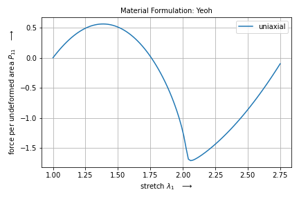
First, setup a problem as usual (mesh, region, field, boundaries and umat). For the material definition we use matADi (pip install madati). We utilize matADi’s lab-capability to visualize the unstable material behavior in uniaxial tension.
# setup a numeric region on a cube
mesh = fem.Cube(n=2)
region = fem.RegionHexahedron(mesh)
field = fem.FieldContainer([fem.Field(region, dim=3)])

# introduce symmetry planes at x=y=z=0
bounds = fem.dof.symmetry(field[0], axes=(True, True, True))

# partition degrees of freedom
dof0, dof1 = fem.dof.partition(field, bounds)

# constitutive isotropic hyperelastic material formulation
yeoh = mat.MaterialHyperelastic(
    mat.models.yeoh, C10=0.5, C20=-0.25, C30=0.025, bulk=5
)

lab = mat.Lab(yeoh)
data = lab.run(
    ux=True,
    bx=False,
    ps=False,
    shear=False,
    stretch_min=1,
    stretch_max=2.75,
    num=100,
)
lab.plot(data)
body = fem.SolidBody(yeoh, field)
An external normal force is applied at \(x=1\) on a quarter model of a cube with symmetry planes at \(x=y=z=0\). Therefore, we have to define an external load vector which will be scaled with the load-proportionality factor \(\lambda\) during numeric continuation.
# external force vector at x=1
right = region.mesh.points[:, 0] == 1
v = 0.01 * region.mesh.cells_per_point[right]
values_load = np.vstack([v, np.zeros_like(v), np.zeros_like(v)]).T

load = fem.PointLoad(field, right, values_load)
The next step involves the problem definition for contique. For details have a look at contique’s README.
def fun(x, lpf, *args):
    "The system vector of equilibrium equations."

    # re-create field-values from active degrees of freedom
    body.field[0].values.fill(0)
    body.field[0].values.ravel()[dof1] += x
    load.update(values_load * lpf)

    return fem.tools.fun([body, load], body.field)[dof1]

def dfundx(x, lpf, *args):
    """The jacobian of the system vector of equilibrium equations w.r.t. the
    primary unknowns."""

    body.field[0].values.fill(0)
    body.field[0].values.ravel()[dof1] += x
    load.update(values_load * lpf)

    r = fem.tools.fun([body, load], body.field, True)
    K = fem.tools.jac([body, load], body.field, True)

    return fem.solve.partition(body.field, K, dof1, dof0, -r)[2]

def dfundl(x, lpf, *args):
    """The jacobian of the system vector of equilibrium equations w.r.t. the
    load proportionality factor."""

    body.field[0].values.fill(0)
    body.field[0].values.ravel()[dof1] += x
    load.update(values_load)

    return load.assemble.vector()[dof1]
Next we have to init the problem and specify the initial values of unknowns (the undeformed configuration). After each completed step of the numeric continuation the XDMF-file will be updated.
# write xdmf file during numeric continuation
with meshio.xdmf.TimeSeriesWriter("result.xdmf") as writer:
    writer.write_points_cells(mesh.points, [(mesh.cell_type, mesh.cells)])

    def step_to_xdmf(step, res):
        writer.write_data(step, point_data={"u": field[0].values})

    # run contique (w/ rebalanced steps, 5% overshoot and a callback function)
    Res = contique.solve(
        fun=fun,
        jac=[dfundx, dfundl],
        x0=field[0][dof1],
        lpf0=0,
        dxmax=0.05,
        dlpfmax=0.5,
        maxsteps=80,
        rebalance=True,
        overshoot=1.05,
        callback=step_to_xdmf,
    )

    X = np.array([res.x for res in Res])
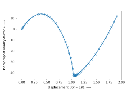
Finally, the force-displacement curve is plotted. It can be seen that the resulting (unstable) force-controlled equilibrium path is equal to the displacement-controlled loadcase of matADi’s lab.
plt.figure()

# plot force-displacement curve
plt.plot(X[:, 0], X[:, -1], "x-")
plt.xlabel(r"displacement $u(x=1)/L$ $\longrightarrow$")
plt.ylabel(r"load-proportionality-factor $\lambda$ $\longrightarrow$")

fem.save(region, field)