Non-homogeneous shear loadcase#
Plane strain hyperelastic non-homogenous shear loadcase
define a non-homogeneous shear loadcase
use a mixed hyperelastic formulation in plane strain
assign a micro-sphere material formulation
define a step and a job along with a callback-function
export and visualize principal stretches
plot force - displacement curves
Two rubber blocks of height \(H\) and length \(L\), both glued to a rigid plate on their top and bottom faces, are subjected to a displacement controlled non-homogeneous shear deformation by \(u_{ext}\) in combination with a compressive normal force \(F\).

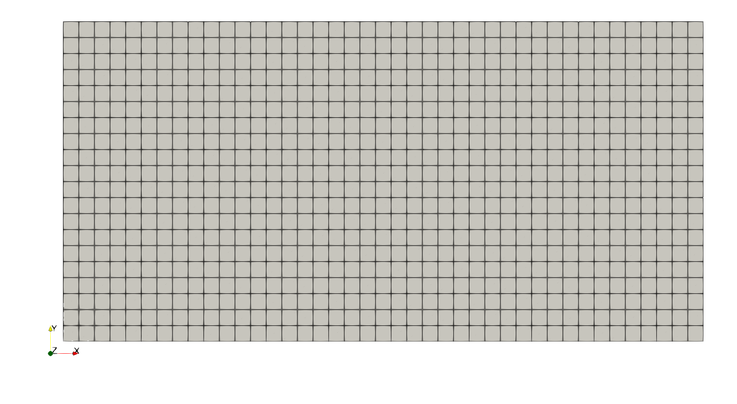
Let’s create the mesh. An additional center-point is created for a multi-point
constraint (MPC). By default, FElupe stores points not connected to any cells in
Mesh.points_without_cells and adds them to the list of inactive
degrees of freedom. Hence, we have to drop our MPC-centerpoint from that list.
import numpy as np
import felupe as fe

H = 10
L = 20
T = 10

n = 21
a = min(L / n, H / n)

mesh = fe.Rectangle((0, 0), (L, H), n=(round(L / a), round(H / a)))
mesh.points = np.vstack((mesh.points, [0, 2 * H]))
mesh.update(mesh.cells)
mesh.points_without_cells = np.array([], dtype=bool)
A numeric quad-region created on the mesh in combination with a vector-valued displacement field for plane-strain as well as scalar-valued fields for the hydrostatic pressure and the volume ratio represents the rubber numerically. A shear loadcase is applied on the displacement field. This involves setting up a y-symmetry plane as well as the absolute value of the prescribed shear movement in direction \(x\) at the MPC-centerpoint.
region = fe.RegionQuad(mesh)
fields = fe.FieldsMixed(region, n=3, planestrain=True)

f0 = lambda y: np.isclose(y, 0)
f2 = lambda y: np.isclose(y, 2* H)

boundaries = {
    "fixed": fe.Boundary(fields[0], fy=f0),
    "control": fe.Boundary(fields[0], fy=f2, skip=(0, 1)),
}

dof0, dof1 = fe.dof.partition(fields, boundaries)
The micro-sphere material formulation is used for the rubber. It is defined as a hyperelastic material in matADi. The material formulation is finally applied on the plane-strain field, resulting in a hyperelastic solid body.
MatADi - Material Definition with Automatic Differentiation
MatADi is a powerful and lightweight Python package for the definition of hyperelastic material model formulations. Do not use the MaterialHyperelasticPlaneStrain() and ThreeFieldVariationPlaneStrain() classes of matADi in combination with a plane-strain field of FElupe. These classes are designed to be used on default two dimensional fields (i.e. use it only with fe.FieldsMixed(region, n=3, planestrain=False). Get matADi on PyPI:
pip install matadi
import matadi as mat

umat = mat.MaterialHyperelastic(
    mat.models.miehe_goektepe_lulei,
    mu=0.1475,
    N=3.273,
    p=9.31,
    U=9.94,
    q=0.567,
    bulk=5000.0,
)

rubber = fe.SolidBody(umat=mat.ThreeFieldVariation(umat), field=fields)
At the centerpoint of a multi-point constraint (MPC) the external shear movement is prescribed. It also ensures a force-free top plate in direction \(y\).
mpc = fe.MultiPointConstraint(
    field=fields,
    points=np.arange(mesh.npoints)[mesh.points[:, 1] == H],
    centerpoint=mesh.npoints - 1,
)
The shear movement is applied in substeps, which are each solved with an iterative newton-rhapson procedure. Inside an iteration, the force residual vector and the tangent stiffness matrix are assembled. The fields are updated with the solution of unknowns. The equilibrium is checked as ratio between the norm of residual forces of the active vs. the norm of the residual forces of the inactive degrees of freedom. If convergence is obtained, the iteration loop ends. Both \(y\)-displacement and the reaction force in direction \(x\) of the top plate are saved. This is realized by a callback-function which is called after each successful substep. A step combines all active items along with constant and ramped boundary conditions. Finally, the step is added to a job. A job returns a generator object with the results of all substeps.
UX = fe.math.linsteps([0, 15], 15)
UY = []
FX = []

def callback(stepnumber, substepnumber, subcase):
    """Callback-function for the evaluation of the force-displacement
    characteristic curves."""

    # get current x-movement
    move = boundaries["control"].value

    UY.append(subcase.x[0].values[mpc.centerpoint, 1])
    FX.append(subcase.fun[2 * mpc.centerpoint] * T)

    print(f"Reaction Force FX(UX) = {FX[-1]:1.1f}N({move}mm)")
    return
step = fe.Step(
    items=[rubber, mpc],
    ramp={boundaries["control"]: UX},
    boundaries=boundaries
)
job = fe.Job(steps=[step], callback=callback)
res = job.evaluate()
For the maximum deformed model a VTK-file containing principal stretches projected to mesh points is exported.
from felupe.math import transpose, dot, eigh

F = fields[0].extract()
C = dot(transpose(F), F)

stretches = fe.project(np.sqrt(eigh(C)[0]), region)

fe.save(region, fields, point_data={
    "Maximum-principal-stretch": np.max(stretches, axis=1),
    "Minimum-principal-stretch": np.min(stretches, axis=1),
})
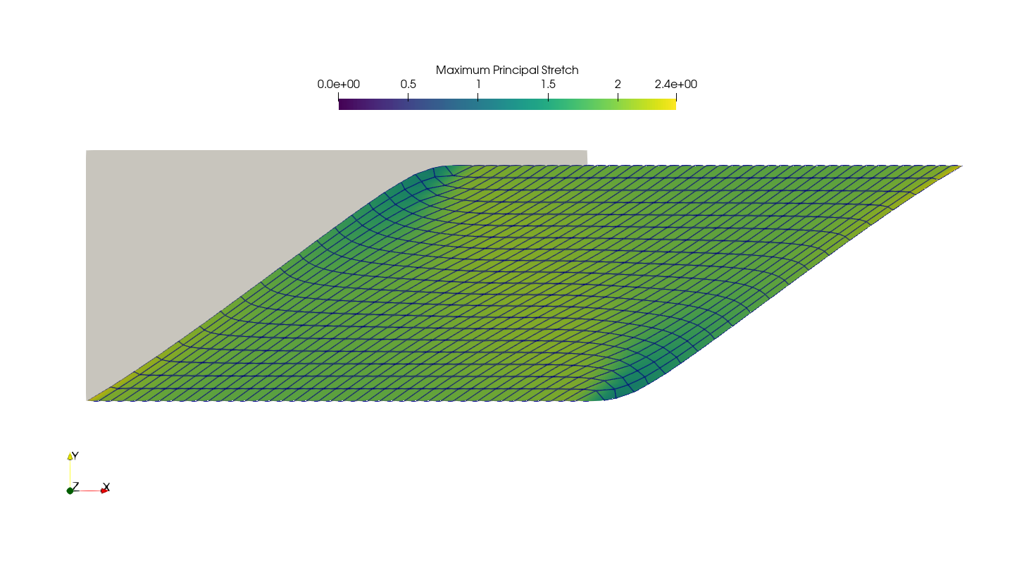
The shear force \(F_x\) vs. the displacements \(u_x\) and \(u_y\), all located at the top plate, are plotted.
import matplotlib.pyplot as plt

fig, ax = plt.subplots(1, 2)

ax[0].plot(UX, FX, 'o-')
ax[0].set_xlim(0, 15)
ax[0].set_ylim(0, 300)
ax[0].set_xlabel(r"$u_x$ in mm")
ax[0].set_ylabel(r"$F_x$ in N")

ax[1].plot(UY, FX, 'o-')
ax[1].set_xlim(-1.2, 0.2)
ax[1].set_ylim(0, 300)
ax[1].set_xlabel(r"$u_y$ in mm")
ax[1].set_ylabel(r"$F_x$ in N")

plt.tight_layout()

plt.savefig("shear_plot.svg")
