FElupe documentation#
FElupe is an open, Python-based finite element infrastructure for nonlinear computational solid mechanics, providing high-level and extensible workflows for research and engineering applications.
New to FElupe? The Beginner’s Guide contains an introduction to the concept of FElupe.
The reference guide contains a detailed description of the FElupe API. It describes how the methods work and which parameters can be used. Requires an understanding of the key concepts.
Step-by-step guides for specific tasks or problems with a focus on practical usability instead of completeness. Requires an understanding of the key concepts.
A gallery of examples.
Highlights
easy to learn and productive high-level API
nonlinear deformation of
solid bodiesinteractive views on meshes, fields and solid bodies (using PyVista)
typical finite elements
cartesian, axisymmetric, plane strain and mixed fields
Installation#
Install Python, open a terminal and run

pip install felupe[all]
where [all] is a combination of [autodiff,io,parallel,plot,progress,view] and installs all optional dependencies. FElupe has minimal requirements, all available at PyPI supporting all platforms.
In order to make use of all features of FElupe, it is suggested to install all optional dependencies.
einsumt for parallel (threaded) assembly
jax for automatic differentiation in material formulations (JAX-based)
h5py for writing XDMF result files
matplotlib for plotting graphs
meshio for mesh-related I/O
pyvista for interactive visualizations
tensortrax for automatic differentiation in material formulations (NumPy-based)
tqdm for showing progress bars during job evaluations
The development version may contain not yet released bug fixes and features. Consider using the --user option to install the package into your home directory (see pip documentation for more details). To install FElupe from the latest development branch, use
pip install git+https://github.com/adtzlr/felupe.git@main
or clone the repository and install the package in editable mode.
git clone https://github.com/adtzlr/felupe.git
cd felupe
pip install --editable .
Optional dependencies may also be installed by replacing the last line.
pip install --editable ".[all]"
Extension Packages#
The capabilities of FElupe may be enhanced with extension packages created by the community.
Package |
Description |
|---|---|
Numerical continuation of nonlinear equilibrium equations. |
|
Constitutive hyperelastic material formulations |
|
Material Definition with Automatic Differentiation (AD) |
|
Snapshot-Driven State Upscaling |
|
Differentiable Tensors based on NumPy Arrays (bundled with FElupe) |
|
A visualization tool for FElupe |
Performance#
This is a simple benchmark to compare assembly times for linear elasticity and hyperelasticity on tetrahedrons.
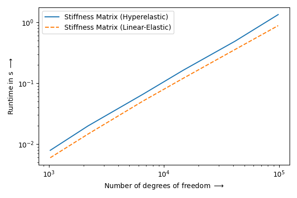
Analysis |
DOF/s |
|---|---|
Linear-Elastic |
130039 +/-23464 |
Hyperelastic |
116819 +/-21979 |
Tested on: Windows 10, Python 3.11, Intel® Core™ i7-11850H @ 2.50GHz, 32GB RAM.
from timeit import timeit

import matplotlib.pyplot as plt
import numpy as np

import felupe as fem


def pre_linear_elastic(n, **kwargs):
    mesh = fem.Cube(n=n).triangulate()
    region = fem.RegionTetra(mesh)
    field = fem.FieldContainer([fem.Field(region, dim=3)])
    umat = fem.LinearElastic(E=1, nu=0.3)
    solid = fem.SolidBody(umat, field)
    return mesh, solid


def pre_hyperelastic(n, **kwargs):
    mesh = fem.Cube(n=n).triangulate()
    region = fem.RegionTetra(mesh)
    field = fem.FieldContainer([fem.Field(region, dim=3)])
    umat = fem.NeoHookeCompressible(mu=1.0, lmbda=2.0)
    solid = fem.SolidBody(umat, field)
    return mesh, solid


print("# Assembly Runtimes")
print("")
print("|   DOF   | Linear-Elastic in s | Hyperelastic in s |")
print("| ------- | ------------------- | ----------------- |")

points_per_axis = np.round((np.logspace(3, 5, 6) / 3)**(1 / 3)).astype(int)

number = 3
parallel = False

runtimes = np.zeros((len(points_per_axis), 2))

for i, n in enumerate(points_per_axis):
    mesh, solid = pre_linear_elastic(n)
    matrix = solid.assemble.matrix(parallel=parallel)
    time_linear_elastic = (
        timeit(lambda: solid.assemble.matrix(parallel=parallel), number=number) / number
    )

    mesh, solid = pre_hyperelastic(n)
    matrix = solid.assemble.matrix(parallel=parallel)
    time_hyperelastic = (
        timeit(lambda: solid.assemble.matrix(parallel=parallel), number=number) / number
    )

    runtimes[i] = time_linear_elastic, time_hyperelastic

    print(
        f"| {mesh.points.size:7d} | {runtimes[i][0]:19.2f} | {runtimes[i][1]:17.2f} |"
    )

dofs_le = points_per_axis ** 3 * 3 / runtimes[:, 0]
dofs_he = points_per_axis ** 3 * 3 / runtimes[:, 1]

print("")
print("| Analysis       |        DOF/s      |")
print("| -------------- | ----------------- |")
print(
    f"| Linear-Elastic |   {np.mean(dofs_le):5.0f} +/-{np.std(dofs_le):5.0f}  |"
)
print(f"| Hyperelastic   |   {np.mean(dofs_he):5.0f} +/-{np.std(dofs_he):5.0f}  |")

plt.figure()
plt.loglog(
    points_per_axis ** 3 * 3,
    runtimes[:, 1],
    "C0",
    label=r"Stiffness Matrix (Hyperelastic)",
)
plt.loglog(
    points_per_axis ** 3 * 3,
    runtimes[:, 0],
    "C1--",
    label=r"Stiffness Matrix (Linear-Elastic)",
)
plt.xlabel(r"Number of degrees of freedom $\longrightarrow$")
plt.ylabel(r"Runtime in s $\longrightarrow$")
plt.legend()
plt.tight_layout()
plt.savefig("benchmark.png")
Contents:
License#
FElupe - Finite Element Analysis (C) 2021-2026 Andreas Dutzler, Graz (Austria).
This program is free software: you can redistribute it and/or modify it under the terms of the GNU General Public License as published by the Free Software Foundation, either version 3 of the License, or (at your option) any later version.
This program is distributed in the hope that it will be useful, but WITHOUT ANY WARRANTY; without even the implied warranty of MERCHANTABILITY or FITNESS FOR A PARTICULAR PURPOSE. See the GNU General Public License for more details.
You should have received a copy of the GNU General Public License along with this program. If not, see https://www.gnu.org/licenses/.