Beginner’s Guide#
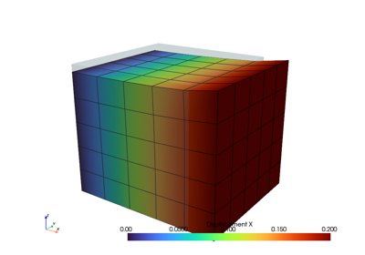
This minimal code-block covers the essential high-level parts of creating and solving problems with FElupe. As an introductory example, a quarter model of a solid cube with hyperelastic material behaviour is subjected to a uniaxial() elongation applied at a clamped end-face.
First, let’s import FElupe and create a meshed cube out of hexahedron cells with a given number of points per axis. A numeric region, pre-defined for hexahedrons, is created on the mesh. A vector-valued displacement field is initiated on the region. Next, a field container is created on top of this field.
import felupe as fem

mesh = fem.Cube(n=6)
region = fem.RegionHexahedron(mesh)
field = fem.FieldContainer([fem.Field(region, dim=3)])
A uniaxial() load case is applied on the displacement field stored inside the field container. This involves setting up symmetry() planes as well as the absolute value of the prescribed displacement at the mesh-points on the right-end face of the cube. The right-end face is clamped: only displacements in direction x are allowed. The dict of boundary conditions for this pre-defined load case are returned as boundaries. Optionally, the partitioned degrees of freedom as well as the external displacements are stored within the returned dict loadcase.
boundaries, loadcase = fem.dof.uniaxial(
    field, clamped=True, return_loadcase=True
)
An isotropic hyperelastic Neo-Hookean material model formulation is applied on the displacement field of a solid body.
umat = fem.NeoHooke(mu=1, bulk=50)
solid = fem.SolidBody(umat, field)
A step generates the consecutive substep-movements of a given boundary condition.
move = fem.math.linsteps([0, 1], num=5)
step = fem.Step(
    items=[solid], ramp={boundaries["move"]: move}, boundaries=boundaries
)
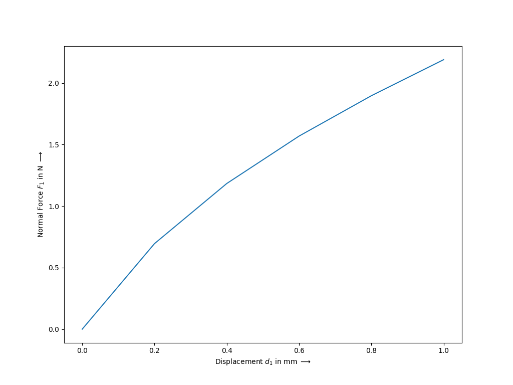
The step is further added to a list of steps of a job. During evaluation, each substep of each step is solved by an iterative Newton-Raphson procedure. The solution is exported after each completed substep as a time-series XDMF file. A characteristic curve plugin is used to record and plot the normal force versus the applied displacement at the right-end face of the cube.
curve = fem.CharacteristicCurvePlugin(boundaries["move"])
job = fem.Job(steps=[step], plugins=[curve])
job.evaluate(filename="result.xdmf")

fig, ax = curve.plot(
    xlabel=r"Displacement $d_1$ in mm $\longrightarrow$",
    ylabel=r"Normal Force $F_1$ in N $\longrightarrow$",
)
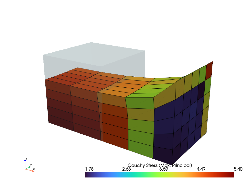
Finally, the result of the last completed substep is plotted.
solid.plot("Principal Values of Cauchy Stress").show()
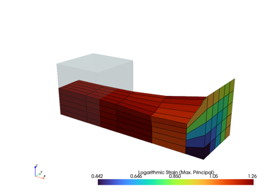
Slightly modified code-blocks are provided for different kind of analyses
and element formulations.
import felupe as fem

mesh = fem.Cube(n=6)
region = fem.RegionHexahedron(mesh)
field = fem.FieldContainer([fem.Field(region, dim=3)])

boundaries = fem.dof.uniaxial(field, clamped=True, return_loadcase=False)

umat = fem.NeoHooke(mu=1, bulk=50)
solid = fem.SolidBody(umat, field)

move = fem.math.linsteps([0, 1], num=5)
step = fem.Step(
    items=[solid], ramp={boundaries["move"]: move}, boundaries=boundaries
)

curve = fem.CharacteristicCurvePlugin(boundaries["move"])
job = fem.Job(steps=[step], plugins=[curve])
job.evaluate()

fig, ax = curve.plot(
    xlabel=r"Displacement $d_1$ in mm $\longrightarrow$",
    ylabel=r"Normal Force $F_1$ in N $\longrightarrow$",
)
solid.plot(
    "Principal Values of Cauchy Stress"
).show()
import felupe as fem

mesh = fem.Cube(n=(9, 5, 5)).add_midpoints_edges()
region = fem.RegionQuadraticHexahedron(mesh)
field = fem.FieldContainer([fem.Field(region, dim=3)])

boundaries = fem.dof.uniaxial(field, clamped=True, return_loadcase=False)

umat = fem.NeoHooke(mu=1, bulk=50)
solid = fem.SolidBody(umat, field)

move = fem.math.linsteps([0, 1], num=5)
step = fem.Step(
    items=[solid], ramp={boundaries["move"]: move}, boundaries=boundaries
)

curve = fem.CharacteristicCurvePlugin(boundaries["move"])
job = fem.Job(steps=[step], plugins=[curve])
job.evaluate()

fig, ax = curve.plot(
    xlabel=r"Displacement $u$ in mm $\longrightarrow$",
    ylabel=r"Normal Force $F$ in N $\longrightarrow$",
)
solid.plot(
    "Principal Values of Cauchy Stress", nonlinear_subdivision=4
).show()
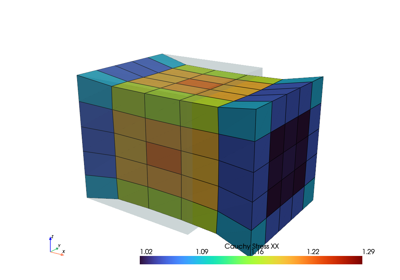
import felupe as fem

mesh = fem.mesh.CubeArbitraryOrderHexahedron(order=3)
region = fem.RegionLagrange(mesh, order=3, dim=3)
field = fem.FieldContainer([fem.Field(region, dim=3)])

boundaries = fem.dof.uniaxial(field, clamped=True, return_loadcase=False)

umat = fem.NeoHooke(mu=1, bulk=50)
solid = fem.SolidBody(umat, field)

move = fem.math.linsteps([0, 1], num=5)
step = fem.Step(
    items=[solid], ramp={boundaries["move"]: move}, boundaries=boundaries
)

curve = fem.CharacteristicCurvePlugin(boundaries["move"])
job = fem.Job(steps=[step], plugins=[curve])
job.evaluate()

fig, ax = curve.plot(
    xlabel=r"Displacement $u$ in mm $\longrightarrow$",
    ylabel=r"Normal Force $F$ in N $\longrightarrow$",
)
solid.plot(
    "Principal Values of Cauchy Stress", project=fem.topoints, nonlinear_subdivision=4
).show()
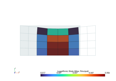
and element formulations.
import felupe as fem

mesh = fem.Rectangle(n=6)
region = fem.RegionQuad(mesh)
field = fem.FieldContainer([fem.FieldPlaneStrain(region, dim=2)])

boundaries = fem.dof.uniaxial(field, clamped=True, return_loadcase=False)

umat = fem.NeoHooke(mu=1, bulk=50)
solid = fem.SolidBody(umat, field)

move = fem.math.linsteps([0, 1], num=5)
step = fem.Step(
    items=[solid], ramp={boundaries["move"]: move}, boundaries=boundaries
)

curve = fem.CharacteristicCurvePlugin(boundaries["move"])
job = fem.Job(steps=[step], plugins=[curve])
job.evaluate()

fig, ax = curve.plot(
    xlabel=r"Displacement $d_1$ in mm $\longrightarrow$",
    ylabel=r"Normal Force $F_1$ in N $\longrightarrow$",
)
solid.plot(
    "Principal Values of Cauchy Stress"
).show()
and element formulations.
import felupe as fem

mesh = fem.Rectangle(n=6)
region = fem.RegionQuad(mesh)
field = fem.FieldContainer([fem.FieldAxisymmetric(region, dim=2)])

boundaries = fem.dof.uniaxial(field, clamped=True, return_loadcase=False)

umat = fem.NeoHooke(mu=1, bulk=50)
solid = fem.SolidBody(umat, field)

move = fem.math.linsteps([0, 1], num=5)
step = fem.Step(
    items=[solid], ramp={boundaries["move"]: move}, boundaries=boundaries
)

curve = fem.CharacteristicCurvePlugin(boundaries["move"])
job = fem.Job(steps=[step], plugins=[curve])
job.evaluate()

fig, ax = job.plot(
    xlabel=r"Displacement $d_1$ in mm $\longrightarrow$",
    ylabel=r"Normal Force $F_1$ in N $\longrightarrow$",
)
solid.plot(
    "Principal Values of Cauchy Stress"
).show()
Tutorials#
This section is all about learning. Each tutorial focuses on some lessons to learn.