Degrees of Freedom#

This module contains the definition of a boundary condition, tools related to the handling of degrees of freedom as well as boundary condition templates for simple load cases.

Core

Boundary(field[, name, fx, fy, fz, value, ...])

A Boundary as a collection of prescribed degrees of freedom (numbered coordinate components of a field at points of a mesh).

Tools

`dof.partition`(field, bounds)	Partition a list of degrees of freedom into prescribed (dof0) and active (dof1) degrees of freedom.
`dof.apply`(field, bounds[, dof0])	Apply prescribed values for a list of boundaries and return all (default) or only the prescribed components of the `field` based on `dof0`.
`dof.symmetry`(field[, axes, x, y, z, bounds])	Return a dict of boundaries for the symmetry axes on the x-, y- and z-coordinates.

Load Cases

`dof.uniaxial`(field[, left, right, move, ...])	Return a dict of boundaries for uniaxial loading between a left (fixed or symmetry face) and a right (applied) end face along a given axis with optional selective symmetries at the origin.
`dof.biaxial`(field[, lefts, rights, moves, ...])	Return a dict of boundaries for biaxial loading between a left (applied or symmetry face) and a right (applied) end face along a given pair of axes with optional selective symmetries at the origin.
`dof.shear`(field[, bottom, top, moves, axes, sym])	Return a dict of boundaries for shear loading with optional combined compression between a rigid bottom and a rigid top end face along a given pair of axes.

Detailed API Reference

class felupe.Boundary(field, name='default', fx=<ufunc 'isnan'>, fy=<ufunc 'isnan'>, fz=<ufunc 'isnan'>, value=0.0, skip=None, mask=None, mode='or')[source]#

A Boundary as a collection of prescribed degrees of freedom (numbered coordinate components of a field at points of a mesh).

Parameters:

field (felupe.Field) – Field on wich the boundary is created.
name (str, optional (default is "default")) – Name of the boundary.
fx (float or callable, optional) – Mask-function for x-component of mesh-points which returns True at points on which the boundary will be applied (default is np.isnan). If a float is passed, this is transformed to lambda x: np.isclose(x, fx).
fy (float or callable, optional) – Mask-function for y-component of mesh-points which returns True at points on which the boundary will be applied (default is np.isnan). If a float is passed, this is transformed to lambda y: np.isclose(y, fy).
fz (float or callable, optional) – Mask-function for z-component of mesh-points which returns True at points on which the boundary will be applied (default is np.isnan). If a float is passed, this is transformed to lambda z: np.isclose(z, fz).
value (ndarray or float, optional) – Value(s) of the selected (prescribed) degrees of freedom (default is 0.0).
skip (None or tuple of bool or int, optional) – A tuple to define which axes of the selected points should be skipped, i.e. not prescribed (default is None and will be set to (False, False, False) if mask=None).
mask (ndarray) – Boolean mask for the prescribed degrees of freedom. If a mask is passed, fx, fy and fz are ignored. However, skip is still applied on the mask.
mode (string, optional) – A string which defines the logical operation for the selected points per axis (default is or).

mask#

1d- or 2d-boolean mask array for the prescribed degrees of freedom.

Type:: ndarray

dof#

1d-array of ints which contains the prescribed degrees of freedom.

Type:: ndarray

points#

1d-array of ints which contains the point ids on which one or more degrees of freedom are prescribed.

Type:: ndarray

value#

Value of the selected (prescribed) degrees of freedom.

Type:: ndarray or float

Examples

A boundary condition prescribes values for chosen degrees of freedom of a given field (not a field container). This is demonstrated for a plane-strain vector field on a quad-mesh of a circle.

>>> import felupe as fem
>>>
>>> mesh = fem.Circle(radius=1, n=6)
>>> x, y = mesh.points.T
>>> region = fem.RegionQuad(mesh)
>>> displacement = fem.FieldPlaneStrain(region, dim=2)
>>> field = fem.FieldContainer([displacement])

A boundary on the displacement field which prescribes all components of the field on the outermost left point of the circle is created. The easiest way is to pass the desired value to fx. The same result is obtained if a callable function is passed to fx.

>>> import numpy as np
>>>
>>> left = fem.Boundary(displacement, fx=x.min())
>>> left = fem.Boundary(displacement, fx=lambda x: np.isclose(x, x.min()))
>>>
>>> plotter = mesh.plot()
>>> actor = plotter.add_points(
...     np.pad(mesh.points[left.points], ((0, 0), (0, 1))),
...     point_size=20,
...     color="red",
... )
>>> plotter.show()

If fx and fy are given, the masks are combined by logical-or.

>>> axes = fem.Boundary(displacement, fx=0, fy=0, mode="or")
>>>
>>> plotter = mesh.plot()
>>> actor = plotter.add_points(
...     np.pad(mesh.points[axes.points], ((0, 0), (0, 1))),
...     point_size=20,
...     color="red",
... )
>>> plotter.show()

This may be changed to logical-and if desired.

>>> center = fem.Boundary(displacement, fx=0, fy=0, mode="and")
>>>
>>> plotter = mesh.plot()
>>> actor = plotter.add_points(
...     np.pad(mesh.points[center.points], ((0, 0), (0, 1))),
...     point_size=20,
...     color="red",
... )
>>> plotter.show()

For the most-general case, a user-defined boolean mask for the selection of the mesh-points is provided. While the two upper methods are useful to select points separated per point-coordinates, providing a mask is more flexible as it may involve all three coordinates (or any other quantities of interest).

>>> mask = np.logical_and(np.isclose(x**2 + y**2, 1), x <= 0)
>>> surface = fem.Boundary(displacement, mask=mask)
>>>
>>> plotter = mesh.plot()
>>> actor = plotter.add_points(
...     np.pad(mesh.points[surface.points], ((0, 0), (0, 1))),
...     point_size=20,
...     color="red",
... )
>>> plotter.show()

The application of a new mask allows to change the selected points of an existing boundary condition.

>>> new_mask = np.logical_and(mask, y >= 0)
>>> surface.apply_mask(new_mask)
>>>
>>> plotter = mesh.plot()
>>> actor = plotter.add_points(
...     np.pad(mesh.points[surface.points], ((0, 0), (0, 1))),
...     point_size=20,
...     color="red",
... )
>>> plotter.show()

A boundary condition may be skipped on given axes, i.e. if only the x-components of a field should be prescribed on the selected points, then the y-axis must be skipped.

>>> axes_x = fem.Boundary(displacement, fx=0, fy=0, skip=(False, True))
>>>
>>> plotter = mesh.plot()
>>> actor = plotter.add_points(
...     np.pad(mesh.points[axes_x.points], ((0, 0), (0, 1))),
...     point_size=20,
...     color="red",
... )
>>> plotter.show()

Values for the prescribed degress of freedom are either applied during creation or by the update-method.

>>> left = fem.Boundary(displacement, fx=x.min(), value=-0.2)
>>> left.update(-0.3)
>>>
>>> plotter = mesh.plot()
>>> actor = plotter.add_points(
...     np.pad(mesh.points[left.points], ((0, 0), (0, 1))),
...     point_size=20,
...     color="red",
... )
>>> plotter.show()

Sometimes it is useful to create a boundary with all axes skipped. This boundary has no prescribed degrees of freedom and hence, is without effect. However, it may still be used in a characteristic job for the boundary to be tracked.

See also

felupe.CharacteristicCurve: A job with a boundary to be tracked.
felupe.dof.partition: Partition degrees of freedom into prescribed and active dof.
felupe.dof.apply: Apply prescribed values for a list of boundaries.

apply_mask(mask)[source]#: Apply a boolean mask to the boundary.

update(value)[source]#: Update the value of the boundary in-place.

felupe.dof.partition(field, bounds)[source]#

Partition a list of degrees of freedom into prescribed (dof0) and active (dof1) degrees of freedom.

Parameters:

field (felupe.FieldContainer) – FieldContainer which holds the fields used in the boundaries.
bounds (dict of felupe.Boundary) – Dict of boundaries.

Returns:

dof0 (ndarray) – 1d-array of int with all prescribed degress of freedom.
dof1 (ndarray) – 1d-array of int with all active degrees of freedom.

Examples

>>> import felupe as fem
>>>
>>> mesh = fem.Rectangle(a=(0, 0), b=(1, 1), n=(3, 3))
>>> region = fem.RegionQuad(mesh)
>>> displacement = fem.FieldPlaneStrain(region, dim=2)
>>> field = fem.FieldContainer([displacement])

A plot shows the point-ids along with the associated degrees of freedom.

>>> plotter = mesh.plot()
>>> actor = plotter.add_point_labels(
...     points=np.pad(mesh.points, ((0, 0), (0, 1))),
...     labels=[
...         f"Point {i}: DOF {a}, {b}"
...         for i, (a, b) in enumerate(displacement.indices.dof)
...     ],
... )
>>> plotter.show()

>>> boundaries = dict(
...     left=fem.Boundary(displacement, fx=0, value=0.2),
...     right=fem.Boundary(displacement, fx=1),
... )
>>> dof0, dof1 = fem.dof.partition(field, boundaries)
>>> dof0
array([ 0,  1,  4,  5,  6,  7, 10, 11, 12, 13, 16, 17])

>>> dof1
array([ 2,  3,  8,  9, 14, 15])

See also

felupe.Boundary: A collection of prescribed degrees of freedom.
felupe.dof.apply: Apply prescribed values for a list of boundaries.

felupe.dof.apply(field, bounds, dof0=None)[source]#

Apply prescribed values for a list of boundaries and return all (default) or only the prescribed components of the field based on dof0.

Parameters:

field (felupe.FieldContainer) – FieldContainer which holds the fields used in the boundaries.
bounds (dict of felupe.Boundary) – Dict of boundaries.
dof0 (ndarray or None, optional) – 1d-array of int with prescribed degrees of freedom (default is None). If not None, only the given deegrees of freedom dof0 of the field values, prescribed by the boundaries, are returned.

Returns:

Field values at mesh-points for all (default) or only the prescribed components of the field based on dof0.

Return type:

ndarray

Examples

>>> import felupe as fem
>>>
>>> mesh = fem.Rectangle(a=(0, 0), b=(1, 1), n=(3, 3))
>>> region = fem.RegionQuad(mesh)
>>> displacement = fem.FieldPlaneStrain(region, dim=2)
>>> field = fem.FieldContainer([displacement])
>>>
>>> boundaries = dict(
...     left=fem.Boundary(displacement, fx=0, value=0.2),
...     right=fem.Boundary(displacement, fx=1),
... )
>>>
>>> dof0, dof1 = fem.dof.partition(field, boundaries)
>>> ext0 = fem.dof.apply(field, boundaries, dof0=dof0)

>>> dof0
array([ 0,  1,  4,  5,  6,  7, 10, 11, 12, 13, 16, 17])

>>> dof1
array([ 2,  3,  8,  9, 14, 15])

>>> ext0
array([0.2, 0.2, 0. , 0. , 0.2, 0.2, 0. , 0. , 0.2, 0.2, 0. , 0. ])

dof0=None is required (default) if the prescribed displacement array should be returned for all degrees of freedom.

>>> fem.dof.apply(field, boundaries).reshape(
...     displacement.values.shape
... )
array([[0.2, 0.2],
       [0. , 0. ],
       [0. , 0. ],
       [0.2, 0.2],
       [0. , 0. ],
       [0. , 0. ],
       [0.2, 0.2],
       [0. , 0. ],
       [0. , 0. ]])

See also

felupe.Boundary: A collection of prescribed degrees of freedom.
felupe.dof.partition: Partition degrees of freedom into prescribed and active dof.

felupe.dof.symmetry(field, axes=(True, True, True), x=0.0, y=0.0, z=0.0, bounds=None)[source]#

Return a dict of boundaries for the symmetry axes on the x-, y- and z-coordinates.

Parameters:

field (felupe.Field) – Field on wich the symmetry boundaries are created.
axes (tuple of bool or int) – Flags to invoke symmetries on the x-, y- and z-axis.
x (float, optional) – Center of the x-symmetry (default is 0.0).
y (float, optional) – Center of the y-symmetry (default is 0.0).
z (float, optional) – Center of the z-symmetry (default is 0.0).
bounds (dict of felupe.Boundary, optional) – Extend a given dict of boundaries by the symmetry boundaries (default is None).

Returns:

New or extended dict of boundaries including symmetry boundaries.

Return type:

dict of felupe.Boundary

Notes

The symmetry boundaries are labeled as "symx", "symy" and "symz".

Symmetry Axis	Prescribed (Fixed) Axes	Skip-Argument
x	y, z	`(True, False, False)`
y	x, z	`(False, True, False)`
z	x, y	`(False, False, True)`

Examples

The x-symmetry boundary for a symmetry on the x-axis contains all points at the given x-coordinate. The degrees of freedom are prescribed except for the symmetry x-axis.

>>> import numpy as np
>>> import felupe as fem
>>>
>>> mesh = fem.Circle(radius=1, n=6, sections=[0, 270])
>>> x, y = mesh.points.T
>>> region = fem.RegionQuad(mesh)
>>> displacement = fem.FieldPlaneStrain(region, dim=2)
>>>
>>> boundaries = fem.dof.symmetry(displacement, axes=(True, False), x=0.0)
>>>
>>> plotter = mesh.plot()
>>> actor = plotter.add_points(
...     np.pad(mesh.points[boundaries["symx"].points], ((0, 0), (0, 1))),
...     point_size=20,
...     color="red",
... )
>>> plotter.show()

See also

felupe.Boundary: A collection of prescribed degrees of freedom.

felupe.dof.uniaxial(field, left=None, right=None, move=0.2, axis=0, clamped=False, sym=True)[source]#

Return a dict of boundaries for uniaxial loading between a left (fixed or symmetry face) and a right (applied) end face along a given axis with optional selective symmetries at the origin. Optionally, the right end face is assumed to be rigid (clamped) in the transversal directions perpendicular to the longitudinal loading direction.

Parameters:

field (felupe.FieldContainer) – FieldContainer on wich the symmetry boundaries are created.
left (float or None, optional) – The position of the left end face along the given axis (default is None). If None, the outermost left position of the mesh-points is taken, i.e. left=field.region.mesh.points[:, axis].min().
right (float or None, optional) – The position of the right end face where the longitudinal movement is applied along the given axis (default is None). If None, the outermost right position of the mesh-points is taken, i.e. right=field.region.mesh.points[:, axis].max().
move (float, optional) – The value of the longitudinal displacement applied at the right end face (default is 0.2).
axis (int, optional) – The longitudinal axis (default is 0).
clamped (bool, optional) – A flag to assume the right end face to be rigid, i.e. zero displacements in the direction of the transversal axes are enforced (default is True).
sym (bool or tuple of bool, optional) – A flag to invoke all (bool) or individual (tuple) symmetry boundaries at the left end face in the direction of the longitudinal axis as well as in the directions of the transversal axes.

Returns:

dict of felupe.Boundary – Dict of boundaries for a uniaxial loadcase.
dict of ndarray – Loadcase-related partitioned prescribed dof0 and active dof1 degrees of freedom as well as the external displacement values ext0 for the prescribed degrees of freedom.

Examples

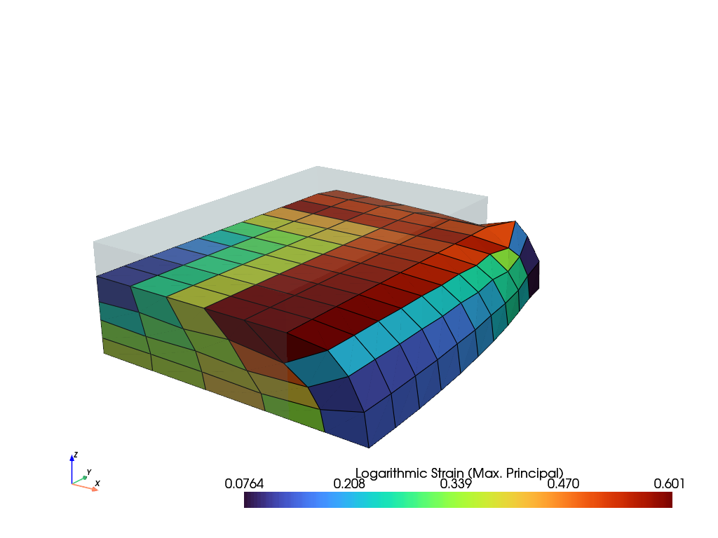
A quarter of a solid hyperelastic cube is subjected to uniaxial displacement- controlled compression on a rigid end face.

>>> import felupe as fem
>>>
>>> region = fem.RegionHexahedron(fem.Cube(a=(0, 0, 0), b=(2, 3, 1), n=(6, 11, 5)))
>>> field = fem.FieldContainer([fem.Field(region, dim=3)])
>>>
>>> boundaries = fem.dof.uniaxial(field, axis=2, clamped=True)[0]

The longitudinal displacement is applied incrementally.

>>> solid = fem.SolidBodyNearlyIncompressible(fem.NeoHooke(mu=1), field, bulk=5000)
>>> step = fem.Step(
...     items=[solid],
...     ramp={boundaries["move"]: fem.math.linsteps([0, -0.3], num=5)},
...     boundaries=boundaries
... )
>>> job = fem.Job(steps=[step]).evaluate()
>>> field.plot("Principal Values of Logarithmic Strain").show()

Static Scene

Interactive Scene

See also

felupe.Boundary: A collection of prescribed degrees of freedom.
felupe.dof.partition: Partition degrees of freedom into prescribed and active dof.
felupe.dof.apply: Apply prescribed values for a list of boundaries.
felupe.dof.symmetry: Return a dict of boundaries for the symmetry axes.

felupe.dof.biaxial(field, lefts=(None, None), rights=(None, None), moves=(0.2, 0.2), axes=(0, 1), clampes=(False, False), sym=True)[source]#

Return a dict of boundaries for biaxial loading between a left (applied or symmetry face) and a right (applied) end face along a given pair of axes with optional selective symmetries at the origin. Optionally, the applied end faces are assumed to be rigid (clamped) in the transversal directions perpendicular to the longitudinal loading direction.

Parameters:

field (felupe.FieldContainer) – FieldContainer on wich the symmetry boundaries are created.
lefts (tuple of float or None, optional) – The position of the left end faces where the longitudinal movement is applied along the given axes (default is (None, None)). If an item of the tuple is None, the outermost left position of the mesh-points is taken, i.e. lefts=[field.region.mesh.points[:, axis].min() for axis in axes].
rights (tuple of float or None, optional) – The position of the right end faces where the longitudinal movement is applied along the given axes (default is (None, None)). If an item of the tuple is None, the outermost right position of the mesh-points is taken, i.e. rights=[field.region.mesh.points[:, axis].max() for axis in axes].
moves (tuple of float, optional) – The values of the longitudinal displacements applied each one half of the value at the left and right end faces (default is (0.2, 0.2)).
axes (tuple of int, optional) – The pair of longitudinal axes (default is (0, 1)).
clampes (tuple of bool, optional) – Flags to assume the applied end faces to be rigid, i.e. zero displacements in the direction of the transversal axes are enforced (default is True).
sym (bool or tuple of bool, optional) – A flag to invoke all (bool) or individual (tuple) symmetry boundaries at the left end face in the directions of the longitudinal axes as well as in the direction of the transversal axis.

Returns:

dict of felupe.Boundary – Dict of boundaries for a biaxial loadcase.
dict of ndarray – Loadcase-related partitioned prescribed dof0 and active dof1 degrees of freedom as well as the external displacement values ext0 for the prescribed degrees of freedom.

Notes

Warning

Note that clampes=(True, True) is not a valid loadcase for a cube. Instead, use a shape where the clamped end faces do not share mesh-points.

Examples

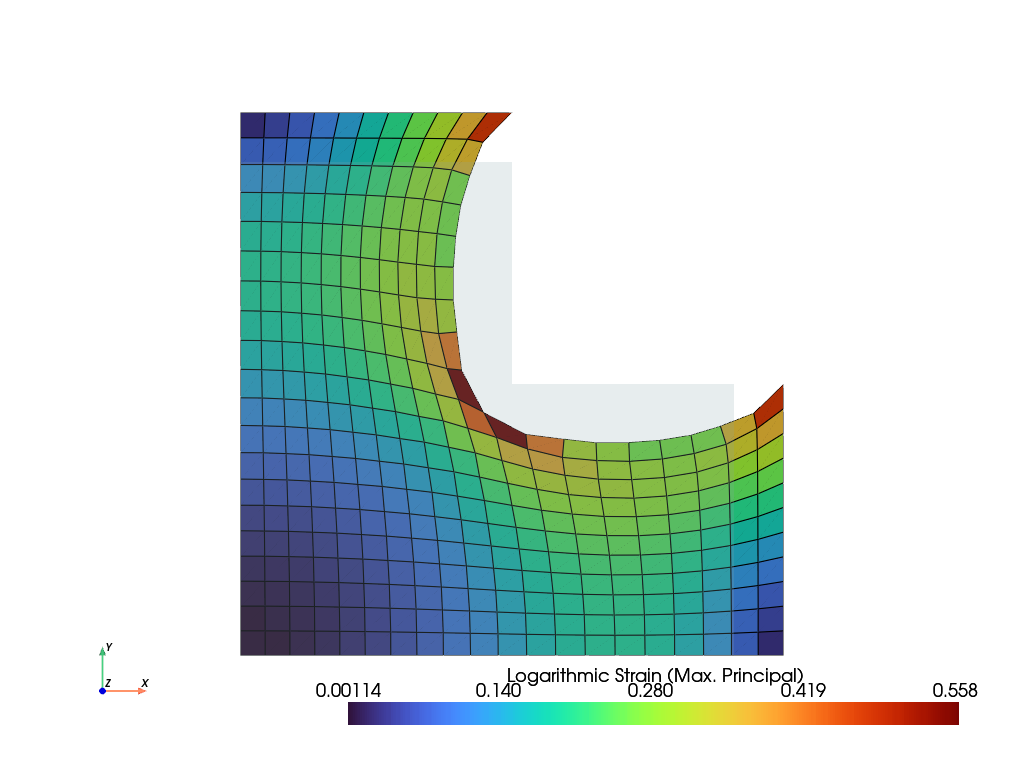
A cross-like planar specimen of a hyperelastic solid is subjected to biaxial displacement-controlled tension on rigid end faces.

>>> import numpy as np
>>> import felupe as fem
>>>
>>> mesh = fem.Rectangle(a=(0, 0), b=(1, 1), n=(21, 21))
>>> x, y = mesh.points.T
>>> points = np.arange(mesh.npoints)[np.logical_or.reduce([x <= 0.6, y <= 0.6])]
>>> mesh.update(cells=mesh.cells[np.all(np.isin(mesh.cells, points), axis=1)])
>>>
>>> region = fem.RegionQuad(mesh)
>>> field = fem.FieldContainer([fem.FieldPlaneStrain(region, dim=2)])
>>>
>>> boundaries = fem.dof.biaxial(field, clampes=(True, True))[0]

The longitudinal displacements are applied incrementally.

>>> solid = fem.SolidBodyNearlyIncompressible(fem.NeoHooke(mu=1), field, bulk=5000)
>>> step = fem.Step(
...     items=[solid],
...     ramp={
...         boundaries["move-right-0"]: fem.math.linsteps([0, 0.1], num=5),
...         boundaries["move-right-1"]: fem.math.linsteps([0, 0.1], num=5),
...     },
...     boundaries=boundaries
... )
>>> job = fem.Job(steps=[step]).evaluate()
>>> field.plot("Principal Values of Logarithmic Strain").show()

Static Scene

Interactive Scene

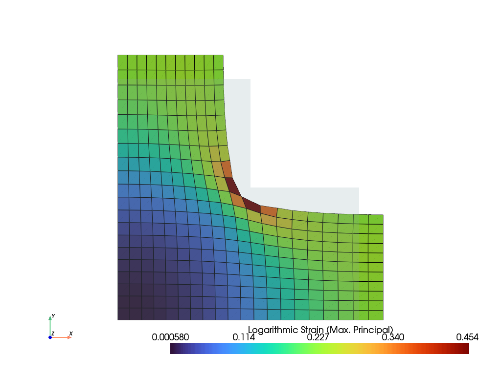
Repeating the above example with fem.dof.biaxial(field, clampes=(False, False) results in a different deformation at the end faces.

>>> import numpy as np
>>> import felupe as fem
>>>
>>> mesh = fem.Rectangle(a=(0, 0), b=(1, 1), n=(21, 21))
>>> x, y = mesh.points.T
>>> points = np.arange(mesh.npoints)[np.logical_or.reduce([x <= 0.6, y <= 0.6])]
>>> mesh.update(cells=mesh.cells[np.all(np.isin(mesh.cells, points), axis=1)])
>>>
>>> region = fem.RegionQuad(mesh)
>>> field = fem.FieldContainer([fem.FieldPlaneStrain(region, dim=2)])
>>>
>>> boundaries = fem.dof.biaxial(field, clampes=(False, False))[0]
>>>
>>> solid = fem.SolidBodyNearlyIncompressible(fem.NeoHooke(mu=1), field, bulk=5000)
>>> step = fem.Step(
...     items=[solid],
...     ramp={
...         boundaries["move-right-0"]: fem.math.linsteps([0, 0.1], num=5),
...         boundaries["move-right-1"]: fem.math.linsteps([0, 0.1], num=5),
...     },
...     boundaries=boundaries
... )
>>> job = fem.Job(steps=[step]).evaluate()
>>> field.plot("Principal Values of Logarithmic Strain").show()

Static Scene

Interactive Scene

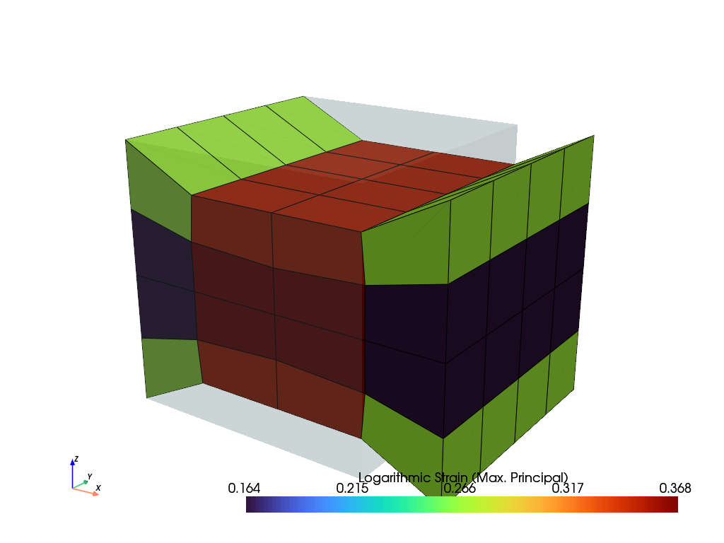
The biaxial load case may also invoke a planar loading, where one of the longitudinal axes is fixed with no displacements at the end plates. The clampling must at least be deactivated on the fixed longitudinal axis.

>>> import felupe as fem
>>>
>>> mesh = fem.Cube(n=5)
>>> region = fem.RegionHexahedron(mesh)
>>> field = fem.FieldContainer([fem.Field(region, dim=3)])
>>> boundaries = fem.dof.biaxial(
...     field, clampes=(True, False), moves=(0, 0), sym=False, axes=(0, 1)
... )[0]
>>> solid = fem.SolidBodyNearlyIncompressible(fem.NeoHooke(mu=1), field, bulk=5000)
>>> step = fem.Step(
...     items=[solid],
...     ramp={boundaries["move-right-0"]: fem.math.linsteps([0, 0.3], num=5),},
...     boundaries=boundaries
... )
>>> job = fem.Job(steps=[step]).evaluate()
>>> field.plot("Principal Values of Logarithmic Strain").show()

Static Scene

Interactive Scene

See also

felupe.Boundary: A collection of prescribed degrees of freedom.
felupe.dof.partition: Partition degrees of freedom into prescribed and active dof.
felupe.dof.apply: Apply prescribed values for a list of boundaries.
felupe.dof.symmetry: Return a dict of boundaries for the symmetry axes.

felupe.dof.shear(field, bottom=None, top=None, moves=(0.2, 0.0, 0.0), axes=(0, 1), sym=True)[source]#

Return a dict of boundaries for shear loading with optional combined compression between a rigid bottom and a rigid top end face along a given pair of axes. The first axis is the direction of shear and the second axis the direction of compression. The bottom face remains fixed while the shear is applied at the top face. Optionally, a symmetry boundary condition in the thickness direction at the origin may be added.

Parameters:

field (felupe.FieldContainer) – FieldContainer on wich the symmetry boundaries are created.
bottom (float or None, optional) – The position of the bottom end face (default is None). If None, the outermost bottom position of the mesh-points is taken, i.e. bottom=[field.region.mesh.points[:, axis].min() for axis in axes].
top (float or None, optional) – The position of the top end face (default is None). If None, the outermost top position of the mesh-points is taken, i.e. top=[field.region.mesh.points[:, axis].min() for axis in axes].
moves (tuple of float, optional) – The values of the displacements applied on the end faces (default is (0.2, 0.0, 0.0)). The first item is the shear displacement applied on the top end face. The second and third items refer to the tension/compression displacements. The second item is applied on the bottom and the third item on the top end face.
axes (tuple of int, optional) – The pair of axes: the first item is the axis of shear and the second item is the axis of compression (default is (0, 1)).
sym (bool, optional) – A flag to invoke a symmetry boundary in the direction of the thickness axis.

Returns:

dict of felupe.Boundary – Dict of boundaries for a biaxial loadcase.
dict of ndarray – Loadcase-related partitioned prescribed dof0 and active dof1 degrees of freedom as well as the external displacement values ext0 for the prescribed degrees of freedom.

Examples

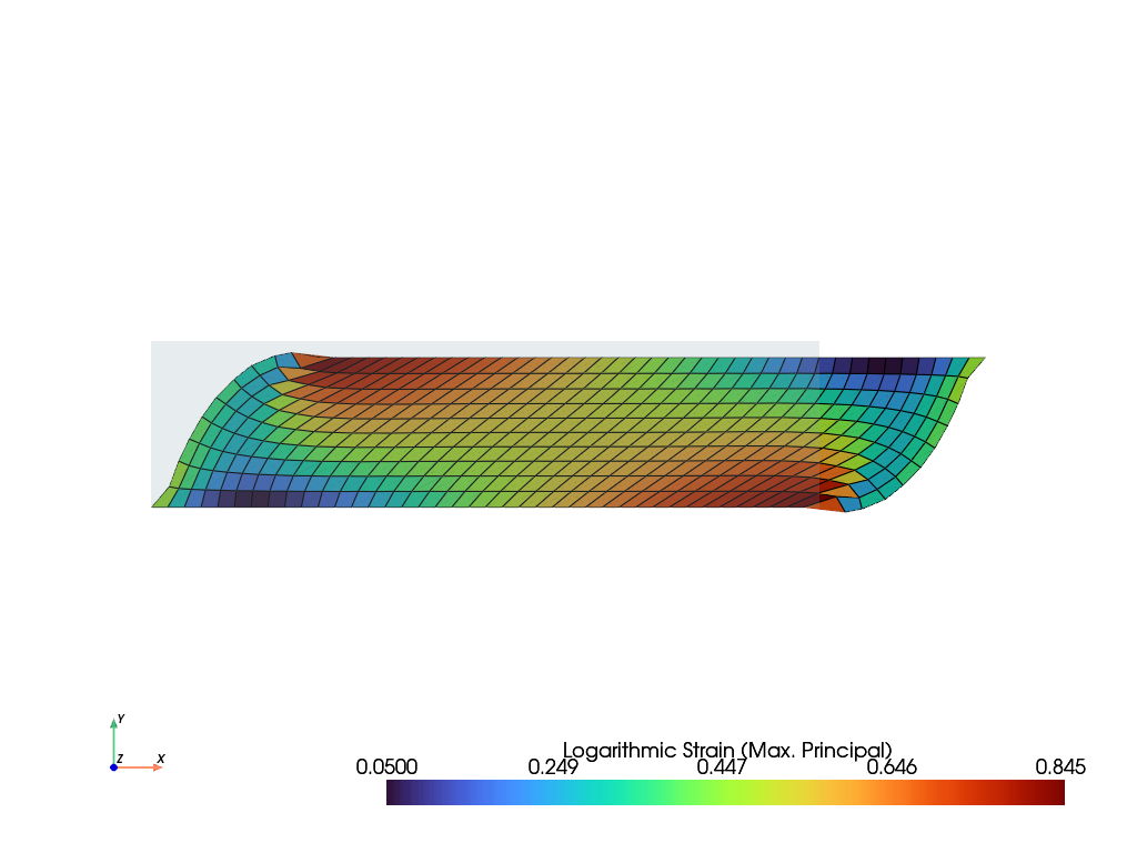
A rectangular planar specimen of a hyperelastic solid is subjected to a displacement-controlled combined shear-compression loading on rigid end faces.

>>> import felupe as fem
>>>
>>> mesh = fem.Rectangle(a=(0, 0), b=(4, 1), n=(41, 11))
>>> region = fem.RegionQuad(mesh)
>>> field = fem.FieldContainer([fem.FieldPlaneStrain(region, dim=2)])

The top edge is moved by -0.1 to add a 10% constant compressive loading.

>>> boundaries = fem.dof.shear(field, moves=(0, 0, -0.1))[0]

The shear displacement is applied incrementally.

>>> solid = fem.SolidBodyNearlyIncompressible(fem.NeoHooke(mu=1), field, bulk=5000)
>>> step = fem.Step(
...     items=[solid],
...     ramp={boundaries["move"]: fem.math.linsteps([0, 1], num=5)},
...     boundaries=boundaries
... )
>>> job = fem.Job(steps=[step]).evaluate()
>>> field.plot("Principal Values of Logarithmic Strain").show()

Static Scene

Interactive Scene

See also

felupe.Boundary: A collection of prescribed degrees of freedom.
felupe.dof.partition: Partition degrees of freedom into prescribed and active dof.
felupe.dof.apply: Apply prescribed values for a list of boundaries.
felupe.dof.symmetry: Return a dict of boundaries for the symmetry axes.