Quadrature#
This module contains quadrature (numeric integration) schemes for different finite element formulations. The integration points of a boundary-quadrature are located on the first edge for 2d elements and on the first face for 3d elements.
Lines, Quads and Hexahedrons
|
An arbitrary-order Gauss-Legendre quadrature rule of dimension 1, 2 or 3 on the interval \([-1, 1]\). |
|
An arbitrary-order Gauss-Legendre quadrature rule of dim 1, 2 or 3 on the interval |
|
An arbitrary-order Gauss-Lobatto quadrature rule of dimension 1, 2 or 3 on the interval \([-1, 1]\). |
|
An arbitrary-order Gauss-Lobatto quadrature rule of dim 1, 2 or 3 on the interval |
Triangles and Tetrahedrons
|
A quadrature scheme suitable for Triangles of order 1, 2 or 3 on the interval \([0, 1]\). |
|
A quadrature scheme suitable for Tetrahedrons of order 1, 2 or 3 on the interval \([0, 1]\). |
|
alias of |
|
alias of |
Sphere
Detailed API Reference
- class felupe.quadrature.Scheme(points, weights)[source]#
Bases:
objectA quadrature scheme with integration points \(x_q\) and weights \(w_q\). It approximates the integral of a function over a region \(V\) by a weighted sum of function values \(f_q = f(x_q)\), evaluated on the quadrature-points.
Notes
The approximation is given by
\[\int_V f(x) dV \approx \sum f(x_q) w_q\]with quadrature points \(x_q\) and corresponding weights \(w_q\).
- plot(plotter=None, point_size=20, weighted=False, **kwargs)[source]#
Plot the quadrature points, scaled by their weights, into a (optionally provided) PyVista plotter.
See also
felupe.Scene.plotPlot method of a scene.
- screenshot(*args, filename=None, transparent_background=None, scale=None, **kwargs)[source]#
Take a screenshot of the quadrature.
See also
pyvista.Plotter.screenshotTake a screenshot of a PyVista plotter.
- class felupe.GaussLegendre(order: int, dim: int, permute: bool = True)[source]#
Bases:
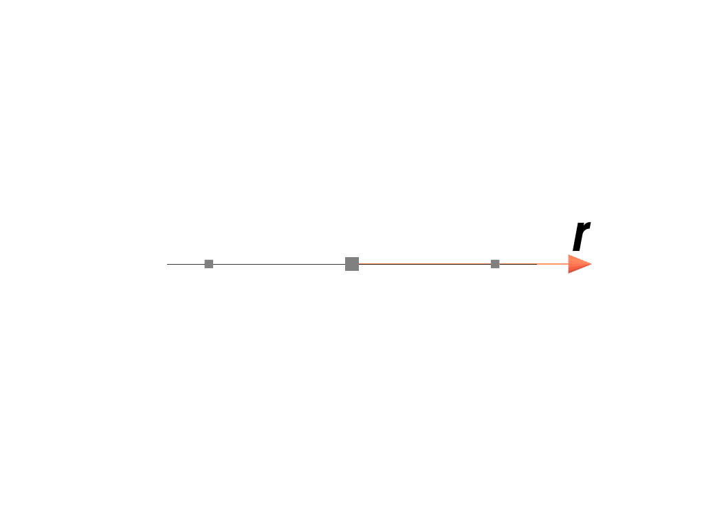
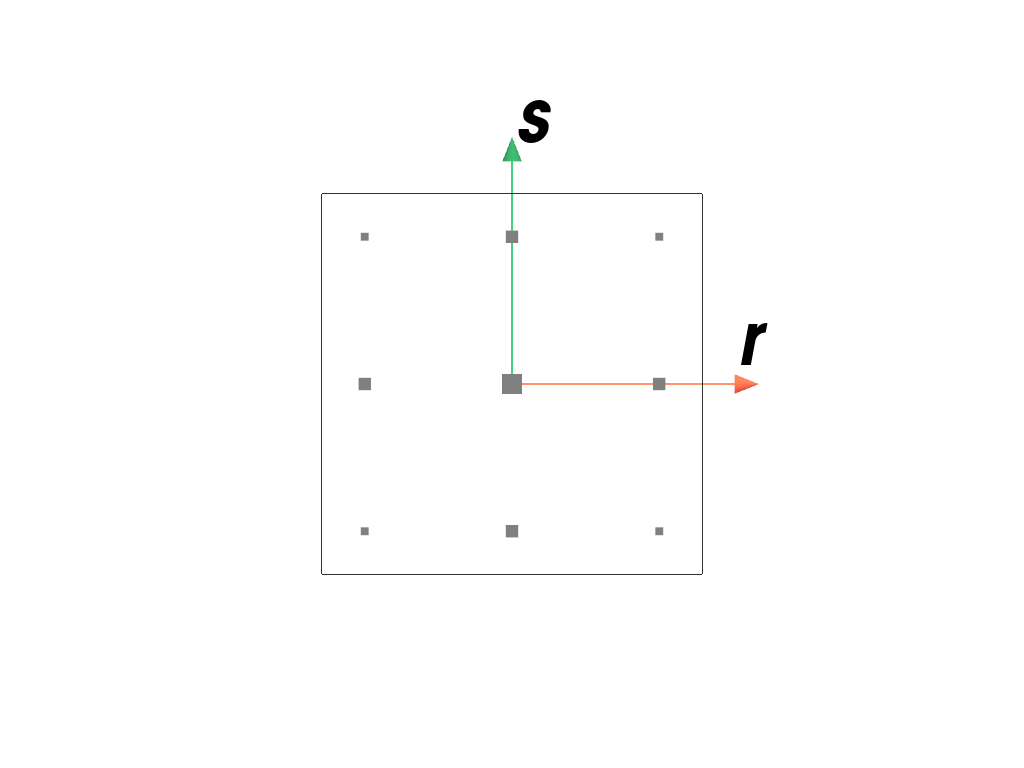
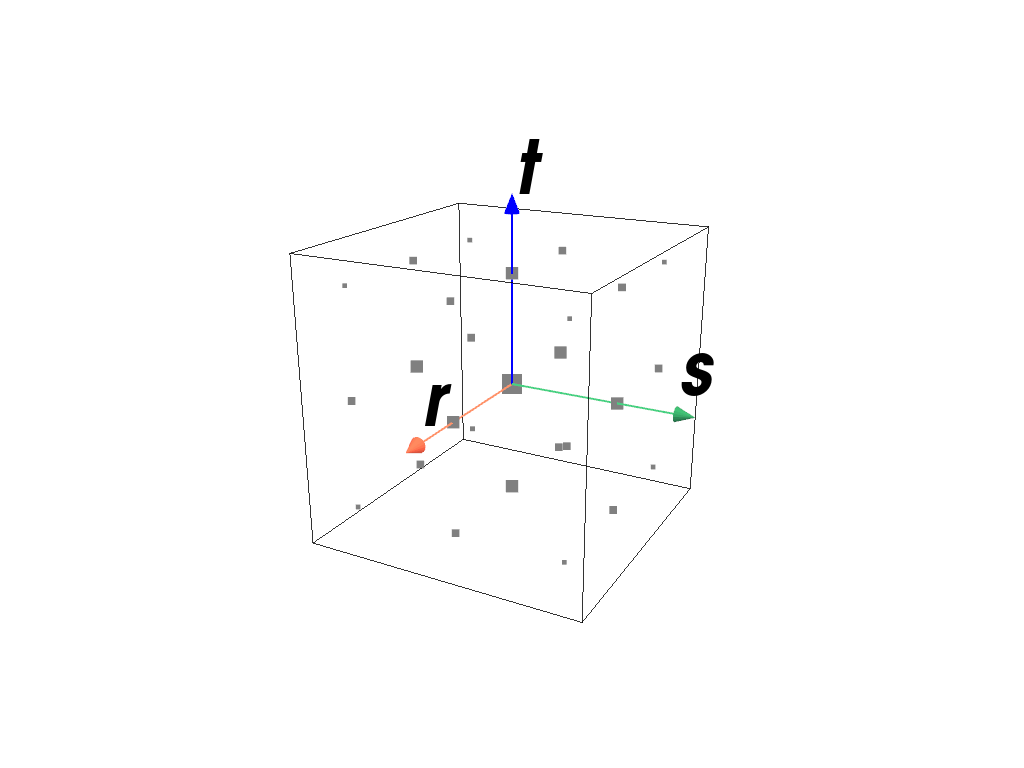
SchemeAn arbitrary-order Gauss-Legendre quadrature rule of dimension 1, 2 or 3 on the interval \([-1, 1]\).
- Parameters:
order (int) – The number of sample points \(n\) minus one. The quadrature rule integrates degree \(2n-1\) polynomials exactly.
dim (int) – The dimension of the quadrature region.
permute (bool, optional) – Permute the quadrature points according to the cell point orderings (default is True). This is supported for two and three dimensions as well as first and second order schemes. Otherwise this flag is silently ignored.
Notes
The approximation is given by
\[\int_{-1}^1 f(x) dx \approx \sum f(x_q) w_q\]with quadrature points \(x_q\) and corresponding weights \(w_q\).
Examples
>>> import felupe as fem
>>>
>>> element = fem.Line()
>>> quadrature = fem.GaussLegendre(order=2, dim=1)
>>> quadrature.plot(
...     plotter=element.plot(add_point_labels=False, show_points=False),
...     weighted=True,
... ).show()
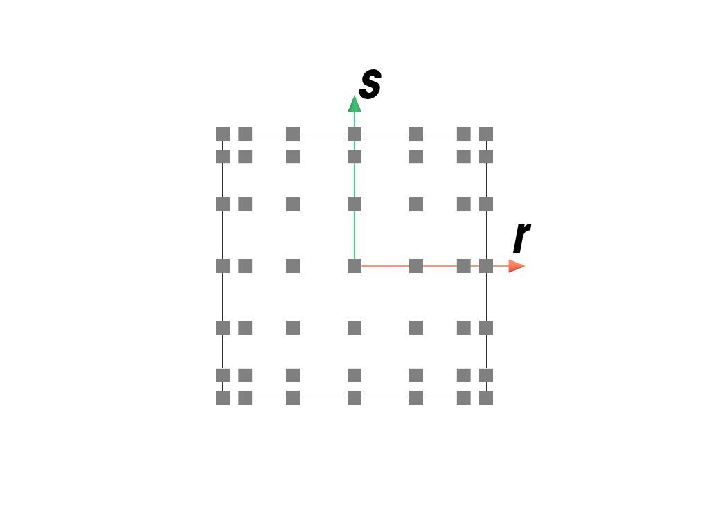
>>> import felupe as fem
>>>
>>> element = fem.QuadraticQuad()
>>> quadrature = fem.GaussLegendre(order=2, dim=2)
>>> quadrature.plot(
...     plotter=element.plot(add_point_labels=False, show_points=False),
...     weighted=True,
... ).show()
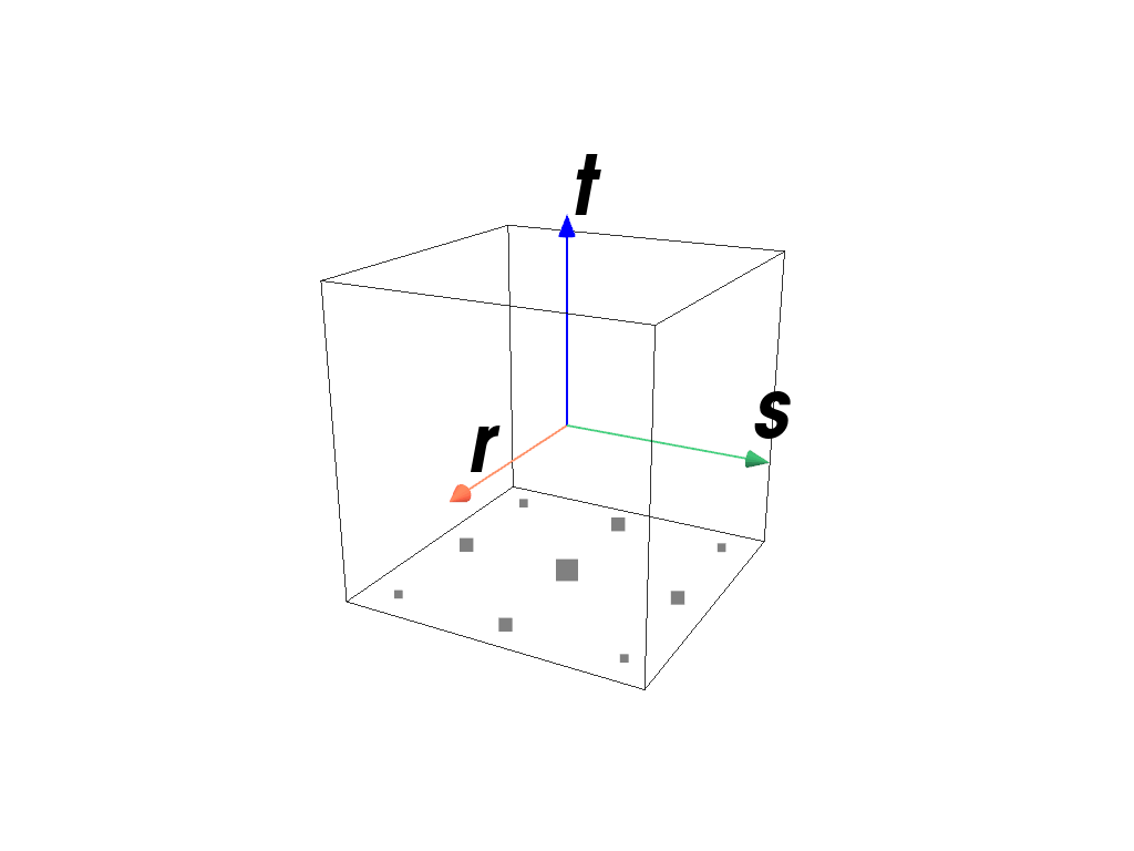
>>> import felupe as fem
>>>
>>> element = fem.QuadraticHexahedron()
>>> quadrature = fem.GaussLegendre(order=2, dim=3)
>>> quadrature.plot(
...     plotter=element.plot(add_point_labels=False, show_points=False),
...     weighted=True,
... ).show()
>>> import felupe as fem
>>>
>>> element = fem.ArbitraryOrderLagrangeElement(order=5, dim=2)
>>> quadrature = fem.GaussLegendre(order=5, dim=2)
>>> quadrature.plot(
...     plotter=element.plot(add_point_labels=False, show_points=False),
...     weighted=True,
... ).show()

- class felupe.GaussLegendreBoundary(order: int, dim: int, permute: bool = True)[source]#
Bases:
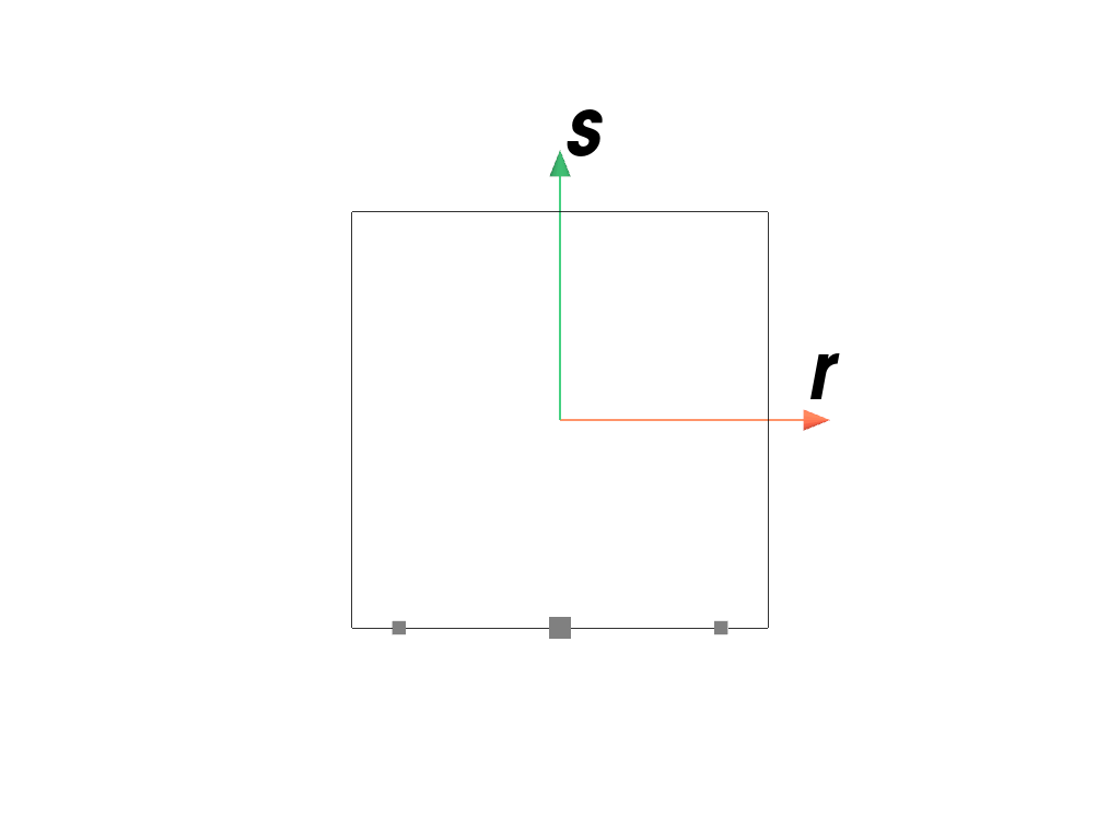
GaussLegendreAn arbitrary-order Gauss-Legendre quadrature rule of dim 1, 2 or 3 on the interval
[-1, 1].- Parameters:
Notes
The approximation is given by
\[\int_{-1}^1 f(x) dx \approx \sum f(x_q) w_q\]with quadrature points \(x_q\) and corresponding weights \(w_q\).
Examples
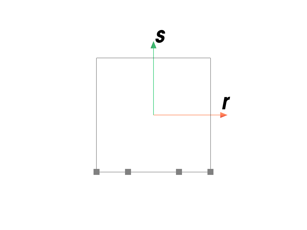
>>> import felupe as fem
>>>
>>> element = fem.QuadraticQuad()
>>> quadrature = fem.GaussLegendreBoundary(order=2, dim=2)
>>> quadrature.plot(
...     plotter=element.plot(add_point_labels=False, show_points=False),
...     weighted=True,
... ).show()
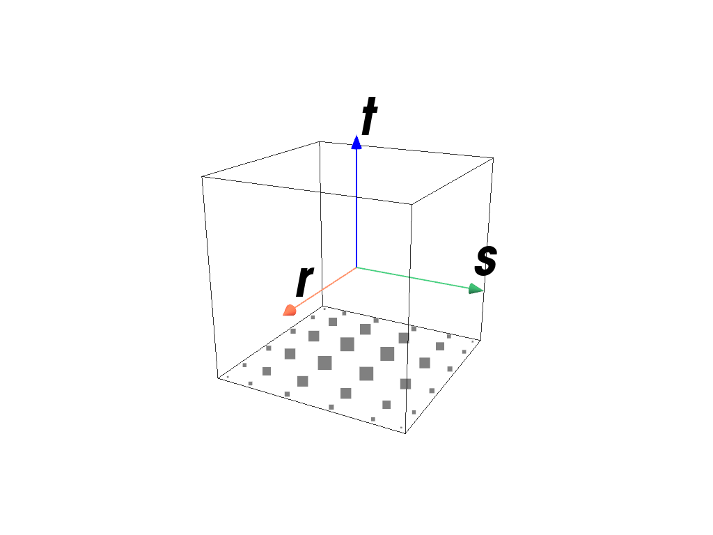
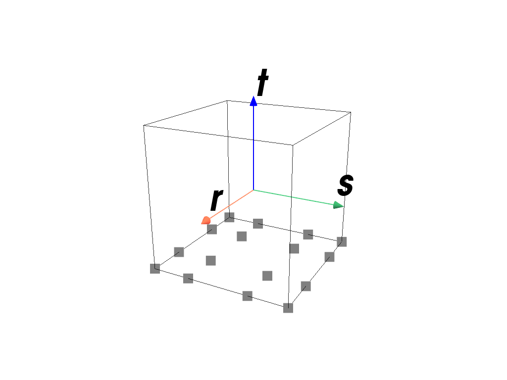
>>> import felupe as fem
>>>
>>> element = fem.QuadraticHexahedron()
>>> quadrature = fem.GaussLegendreBoundary(order=2, dim=3)
>>> quadrature.plot(
...     plotter=element.plot(add_point_labels=False, show_points=False),
...     weighted=True,
... ).show()
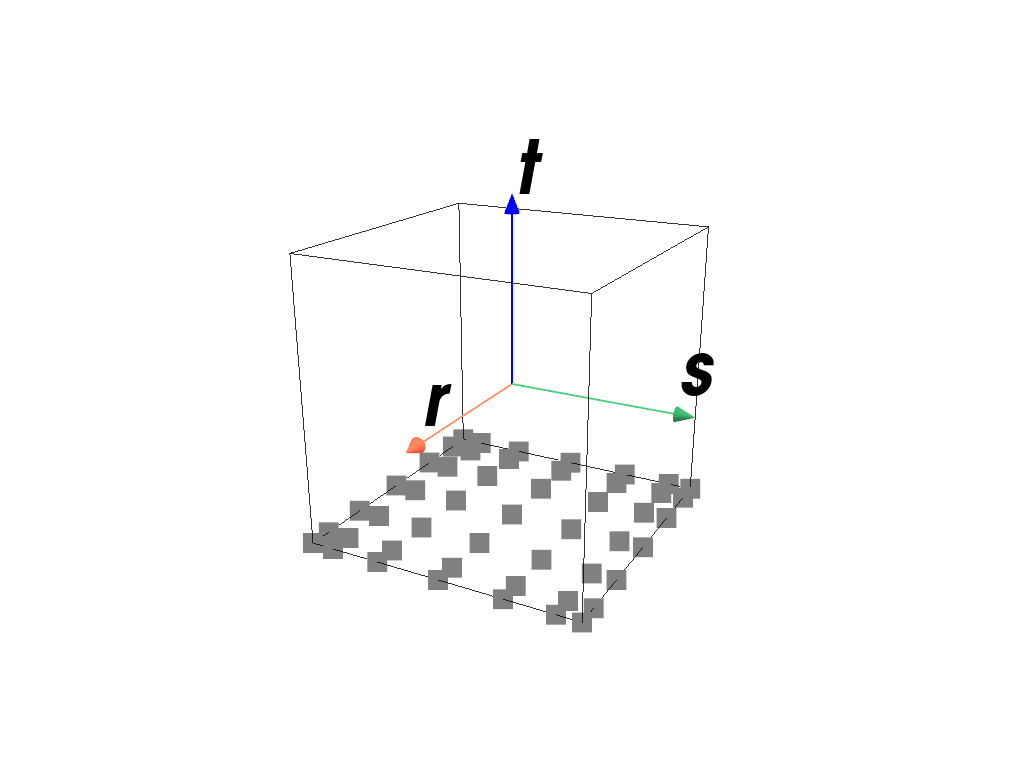
>>> import felupe as fem
>>>
>>> element = fem.ArbitraryOrderLagrangeElement(order=5, dim=3)
>>> quadrature = fem.GaussLegendreBoundary(order=5, dim=3)
>>> quadrature.plot(
...     plotter=element.plot(add_point_labels=False, show_points=False),
...     weighted=True,
... ).show()
- class felupe.GaussLobatto(order: int, dim: int)[source]#
Bases:
SchemeAn arbitrary-order Gauss-Lobatto quadrature rule of dimension 1, 2 or 3 on the interval \([-1, 1]\).
- Parameters:
order (int) – The number of sample points \(n\) minus two. The quadrature rule integrates degree \(2n-3\) polynomials exactly.
dim (int) – The dimension of the quadrature region.
permute (bool, optional) – Permute the quadrature points according to the cell point orderings (default is True). This is supported for two and three dimensions as well as first and second order schemes. Otherwise this flag is silently ignored.
Notes
The approximation is given by
\[\int_{-1}^1 f(x) dx \approx \sum f(x_q) w_q\]with quadrature points \(x_q\) and corresponding weights \(w_q\).
Examples
Note
The quadrature points are not weighted in the plots because the end-points would be almost invisible for the Gauss-Lobatto quadrature rule.
>>> import felupe as fem
>>>
>>> element = fem.Line()
>>> quadrature = fem.GaussLobatto(order=2, dim=1)
>>> quadrature.plot(
...     plotter=element.plot(add_point_labels=False, show_points=False),
...     weighted=False,
... ).show()

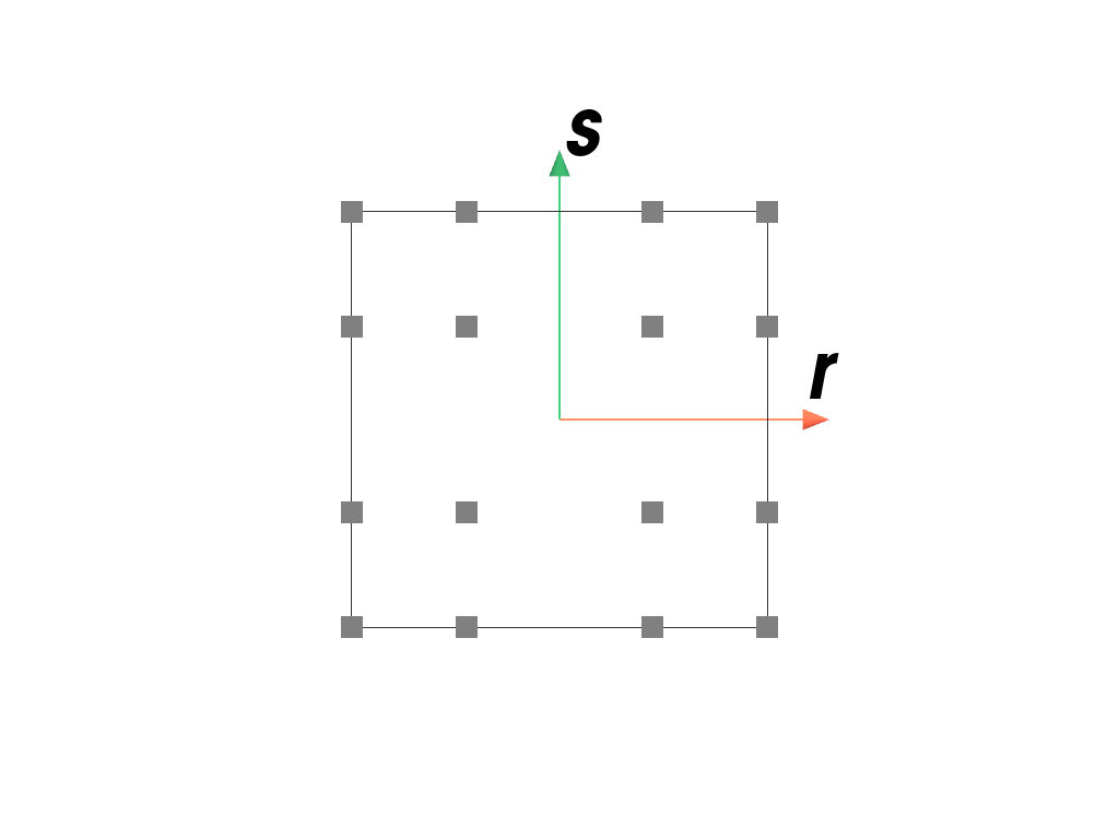
>>> import felupe as fem
>>>
>>> element = fem.QuadraticQuad()
>>> quadrature = fem.GaussLobatto(order=2, dim=2)
>>> quadrature.plot(
...     plotter=element.plot(add_point_labels=False, show_points=False),
...     weighted=False,
... ).show()
>>> import felupe as fem
>>>
>>> element = fem.QuadraticHexahedron()
>>> quadrature = fem.GaussLobatto(order=2, dim=3)
>>> quadrature.plot(
...     plotter=element.plot(add_point_labels=False, show_points=False),
...     weighted=False,
... ).show()
>>> import felupe as fem
>>>
>>> element = fem.ArbitraryOrderLagrangeElement(order=5, dim=2)
>>> quadrature = fem.GaussLobatto(order=5, dim=2)
>>> quadrature.plot(
...     plotter=element.plot(add_point_labels=False, show_points=False),
...     weighted=False,
... ).show()
- class felupe.GaussLobattoBoundary(order: int, dim: int)[source]#
Bases:
GaussLobattoAn arbitrary-order Gauss-Lobatto quadrature rule of dim 1, 2 or 3 on the interval
[-1, 1].- Parameters:
Notes
The approximation is given by
\[\int_{-1}^1 f(x) dx \approx \sum f(x_q) w_q\]with quadrature points \(x_q\) and corresponding weights \(w_q\).
Examples
Note
The quadrature points are not weighted in the plots because the end-points would be almost invisible for the Gauss-Lobatto quadrature rule.
>>> import felupe as fem
>>>
>>> element = fem.QuadraticQuad()
>>> quadrature = fem.GaussLobattoBoundary(order=2, dim=2)
>>> quadrature.plot(
...     plotter=element.plot(add_point_labels=False, show_points=False),
...     weighted=False,
... ).show()
>>> import felupe as fem
>>>
>>> element = fem.QuadraticHexahedron()
>>> quadrature = fem.GaussLobattoBoundary(order=2, dim=3)
>>> quadrature.plot(
...     plotter=element.plot(add_point_labels=False, show_points=False),
...     weighted=False,
... ).show()
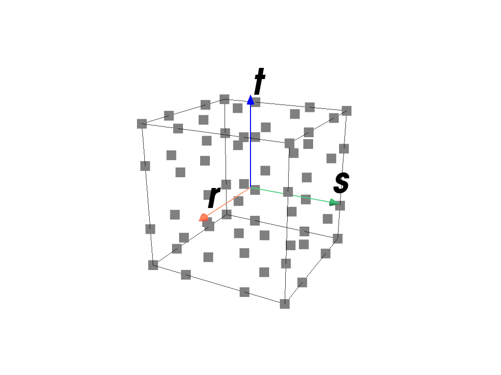
>>> import felupe as fem
>>>
>>> element = fem.ArbitraryOrderLagrangeElement(order=5, dim=3)
>>> quadrature = fem.GaussLobattoBoundary(order=5, dim=3)
>>> quadrature.plot(
...     plotter=element.plot(add_point_labels=False, show_points=False),
...     weighted=False,
... ).show()
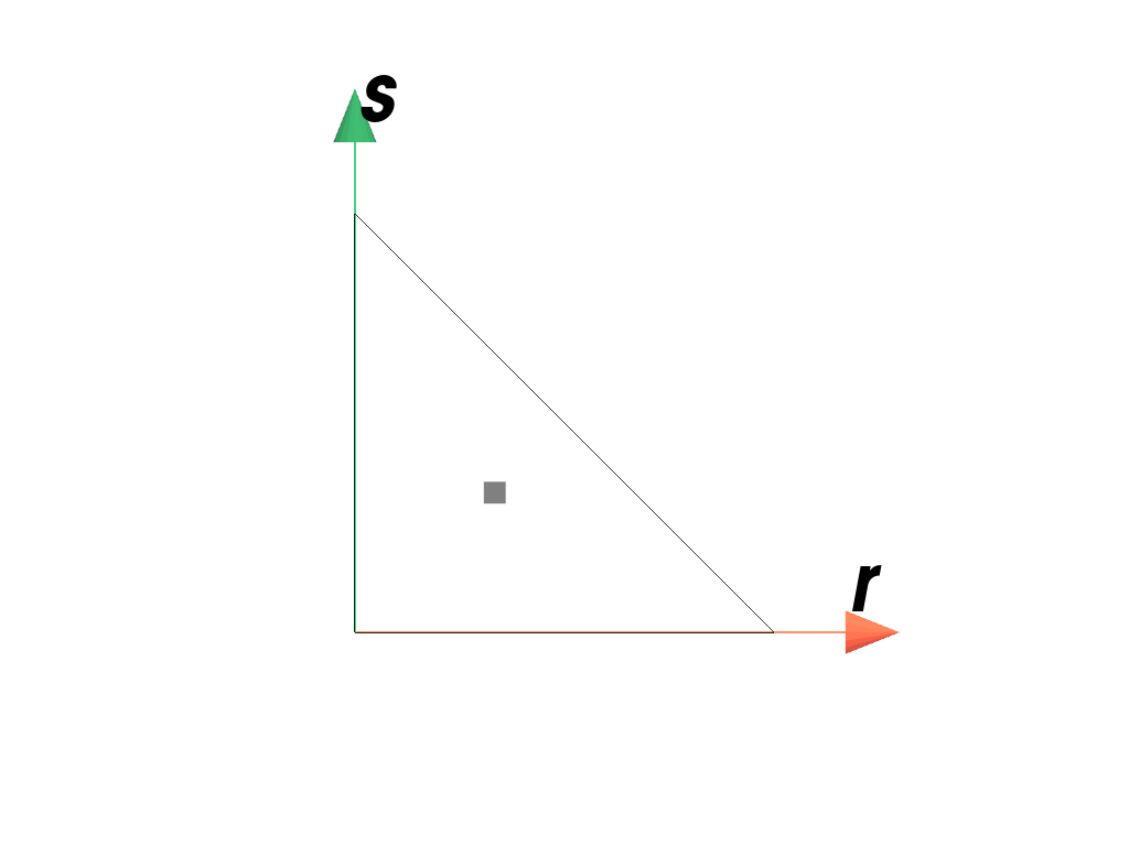
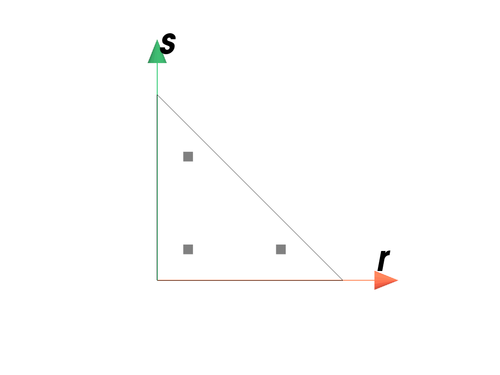
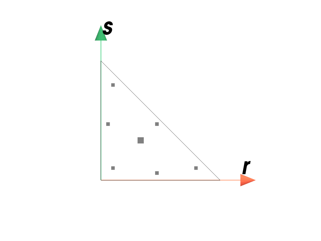
- class felupe.quadrature.Triangle(order: int)[source]#
Bases:
SchemeA quadrature scheme suitable for Triangles of order 1, 2 or 3 on the interval \([0, 1]\).
- Parameters:
order (int) – The order of the quadrature scheme.
Notes
The approximation is given by
\[\int_A f(x) dA \approx \sum f(x_q) w_q\]with quadrature points \(x_q\) and corresponding weights \(w_q\) [1]_ [2].
Examples
>>> import felupe as fem
>>>
>>> element = fem.Triangle()
>>> quadrature = fem.TriangleQuadrature(order=1)
>>> quadrature.plot(
...     plotter=element.plot(add_point_labels=False, show_points=False),
...     weighted=True,
... ).show()
>>> import felupe as fem
>>>
>>> element = fem.QuadraticTriangle()
>>> quadrature = fem.TriangleQuadrature(order=2)
>>> quadrature.plot(
...     plotter=element.plot(add_point_labels=False, show_points=False),
...     weighted=True,
... ).show()
>>> import felupe as fem
>>>
>>> element = fem.QuadraticTriangle()
>>> quadrature = fem.TriangleQuadrature(order=5)
>>> quadrature.plot(
...     plotter=element.plot(add_point_labels=False, show_points=False),
...     weighted=True,
... ).show()
References
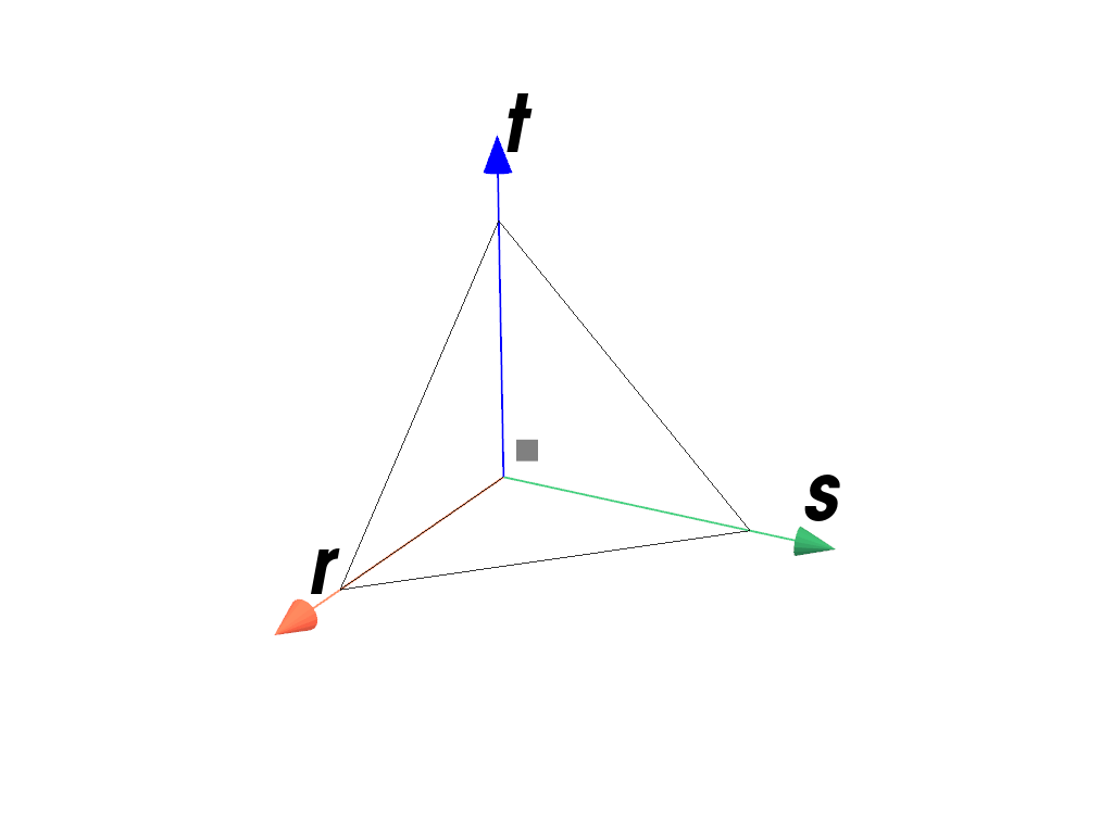
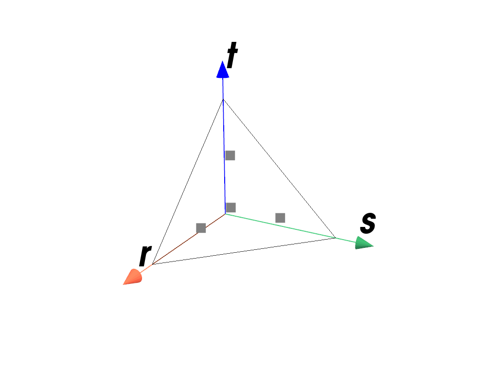
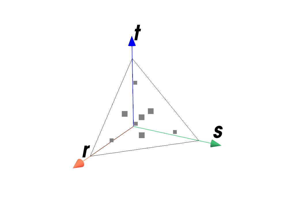
- class felupe.quadrature.Tetrahedron(order: int)[source]#
Bases:
SchemeA quadrature scheme suitable for Tetrahedrons of order 1, 2 or 3 on the interval \([0, 1]\).
- Parameters:
order (int) – The order of the quadrature scheme.
Notes
The approximation is given by
\[\int_V f(x) dV \approx \sum f(x_q) w_q\]with quadrature points \(x_q\) and corresponding weights \(w_q\) [1]_.
Examples
>>> import felupe as fem
>>>
>>> element = fem.Tetra()
>>> quadrature = fem.TetrahedronQuadrature(order=1)
>>> quadrature.plot(
...     plotter=element.plot(add_point_labels=False, show_points=False),
...     weighted=True,
... ).show()
>>> import felupe as fem
>>>
>>> element = fem.QuadraticTetra()
>>> quadrature = fem.TetrahedronQuadrature(order=2)
>>> quadrature.plot(
...     plotter=element.plot(add_point_labels=False, show_points=False),
...     weighted=True,
... ).show()
>>> import felupe as fem
>>>
>>> element = fem.QuadraticTetra()
>>> quadrature = fem.TetrahedronQuadrature(order=5)
>>> quadrature.plot(
...     plotter=element.plot(add_point_labels=False, show_points=False),
...     weighted=True,
... ).show()
References
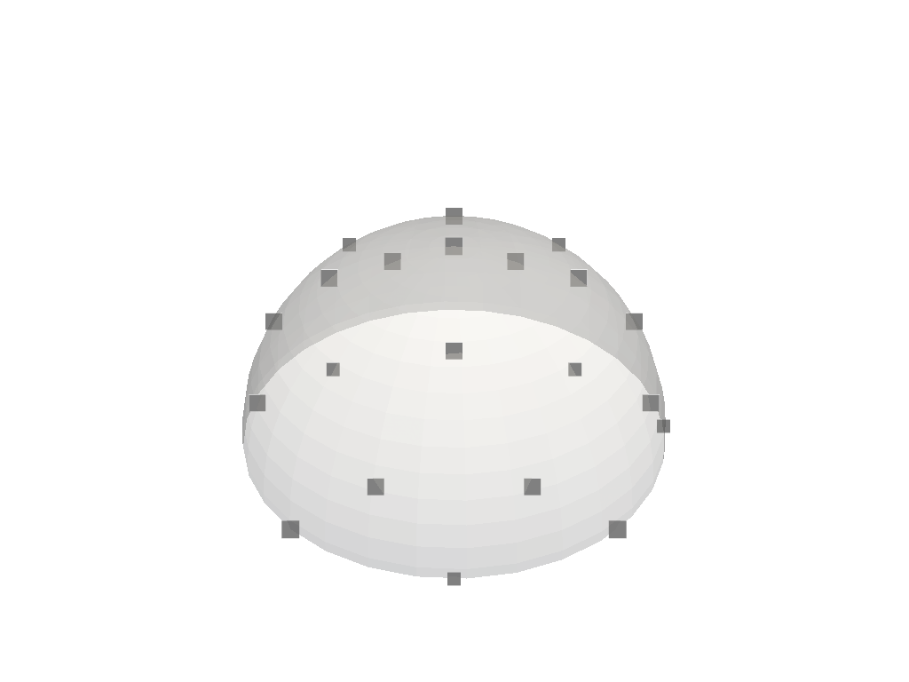
- class felupe.BazantOh(n: int = 21)[source]#
Bases:
SchemeQuadrature scheme for a numeric integration of the surface of a unit sphere [1]_.
- Parameters:
n (int, optional) – The number of quadrature points (default is 21).
Notes
The approximation is given by
\[\int_{\partial V} f(x) dA \approx \sum f(x_q) w_q\]with quadrature points \(x_q\) and corresponding weights \(w_q\).
Examples
>>> import felupe as fem
>>> import pyvista as pv
>>>
>>> plotter = pv.Plotter()
>>> sphere = pv.Sphere(radius=1).clip(normal="z", invert=False)
>>> actor = plotter.add_mesh(sphere, opacity=0.3, color="white")
>>>
>>> quadrature = fem.BazantOh(n=21)
>>> quadrature.plot(plotter=plotter, weighted=True).show()
References