Mechanics#

Solid Bodies

`SolidBody`(umat, field[, statevars])	A SolidBody with methods for the assembly of sparse vectors/matrices.
`SolidBodyNearlyIncompressible`(umat, field, bulk)	A (nearly) incompressible solid body with methods for the assembly of sparse vectors/matrices.
`SolidBodyPressure`(field[, pressure])	A hydrostatic pressure boundary on a solid body.
`SolidBodyGravity`(field[, gravity, density])	A gravity (body) force on a solid body.

State Variables

StateNearlyIncompressible(field)

A State with internal cell-wise constant dual fields for (nearly) incompressible solid bodies.

Steps and Jobs

`Step`(items[, ramp, boundaries])	A Step with multiple substeps, subsequently depending on the solution of the previous substep.
`Job`(steps[, callback])	A job with a list of steps and a method to evaluate them.
`CharacteristicCurve`(steps, boundary[, ...])	A job with a list of steps and a method to evaluate them.

Point Load and Multi-Point Constraints

`PointLoad`(field, points[, values, apply_on, ...])	A point load with methods for the assembly of sparse vectors/matrices.
`MultiPointConstraint`(field, points, centerpoint)
`MultiPointContact`(field, points, centerpoint)

Detailed API Reference

class felupe.SolidBody(umat, field, statevars=None)[source]#

Bases: Solid

A SolidBody with methods for the assembly of sparse vectors/matrices.

Parameters:

umat (class) – A class which provides methods for evaluating the gradient and the hessian of the strain energy density function per unit undeformed volume. The function signatures must be dψdF, ζ_new = umat.gradient([F, ζ]) for the gradient and d2ψdFdF = umat.hessian([F, ζ]) for the hessian of the strain energy density function \(\psi(\boldsymbol{F})\), where \(\boldsymbol{F}\) is the deformation gradient tensor and \(\zeta\) holds the array of internal state variables.
field (FieldContainer) – A field container with one or more fields.
statevars (ndarray or None, optional) – Array of initial internal state variables (default is None).

Notes

The total potential energy of internal forces is given in Eq. (1)

(1)#\[\Pi_{int}(\boldsymbol{F}) = \int_V \psi(\boldsymbol{F})\ dV\]

with its variation, see Eq. (2)

(2)#\[\delta_\boldsymbol{u}(\Pi_{int}) = \int_V \frac{\partial \psi}{\partial \boldsymbol{F}} \ dV \longrightarrow \boldsymbol{f}_\boldsymbol{u}\]

and linearization, see Eq. (3). The right-arrows in Eq. (2) and Eq. (3) represent the assembly into system scalars, vectors or matrices.

(3)#\[\delta_\boldsymbol{u}\Delta_\boldsymbol{u}(\Pi_{int}) = \int_V \delta\boldsymbol{F} : \frac{\partial^2 \psi}{ \partial \boldsymbol{F}\ \partial \boldsymbol{F} } : \Delta\boldsymbol{F}\ dV \longrightarrow \boldsymbol{K}_{\boldsymbol{u}\boldsymbol{u}}\]

The displacement-based formulation leads to a linearized equation system as given in Eq. (4).

(4)#\[\boldsymbol{K}_{\boldsymbol{u}\boldsymbol{u}} \cdot \delta \boldsymbol{u} + \boldsymbol{f}_\boldsymbol{u} = \boldsymbol{0}\]

Note

This class also supports umat with mixed-field formulations like NearlyIncompressible or ThreeFieldVariation.

Examples

>>> import felupe as fem
>>>
>>> mesh = fem.Cube(n=6)
>>> region = fem.RegionHexahedron(mesh)
>>> field = fem.FieldContainer([fem.Field(region, dim=3)])
>>> boundaries, loadcase = fem.dof.uniaxial(field, clamped=True)
>>>
>>> umat = fem.NeoHooke(mu=1, bulk=2)
>>> solid = fem.SolidBody(umat, field)
>>>
>>> table = fem.math.linsteps([0, 1], num=5)
>>> step = fem.Step(
...     items=[solid],
...     ramp={boundaries["move"]: table},
...     boundaries=boundaries,
... )
>>>
>>> job = fem.Job(steps=[step]).evaluate()
>>> solid.plot("Principal Values of Cauchy Stress").show()

Static Scene

Interactive Scene

See also

felupe.SolidBodyNearlyIncompressible: A (nearly) incompressible solid body with methods for the assembly of sparse vectors/matrices.

class felupe.SolidBodyNearlyIncompressible(umat, field, bulk, state=None, statevars=None)[source]#

Bases: Solid

A (nearly) incompressible solid body with methods for the assembly of sparse vectors/matrices. The constitutive material definition must provide the distortional part of the strain energy density function per unit undeformed volume only. The volumetric part of the strain energy density function is automatically added on additonal internal (dual) cell-wise constant fields.

Parameters:

umat (class) – A class which provides methods for evaluating the gradient and the hessian of the isochoric part of the strain energy density function per unit undeformed volume \(\hat\psi(\boldsymbol{F})\). The function signatures must be dψdF, ζ_new = umat.gradient([F, ζ]) for the gradient and d2ψdFdF = umat.hessian([F, ζ]) for the hessian of the strain energy density function \(\hat{\psi}(\boldsymbol{F})\), where \(\boldsymbol{F}\) is the deformation gradient tensor and \(\zeta\) holds the array of internal state variables.
field (FieldContainer) – A field container with one or more fields.
bulk (float) – The bulk modulus of the volumetric part of the strain energy function \(U(\bar{J})=K(\bar{J}-1)^2/2\).
state (StateNearlyIncompressible or None, optional) – A valid initial state for a (nearly) incompressible solid (default is None).
statevars (ndarray or None, optional) – Array of initial internal state variables (default is None).

Notes

The total potential energy of internal forces for a three-field variational approach, suitable for nearly-incompressible material behaviour, is given in Eq. (5)

(5)#\[\Pi_{int}(\boldsymbol{F}, p, \bar{J}) = \int_V \hat{\psi}(\boldsymbol{F})\ dV + \int_V U(\bar{J})\ dV + \int_V p (J - \bar{J})\ dV\]

with its variations, see Eq. (6)

(6)#\[ \begin{align}\begin{aligned}\delta_\boldsymbol{u}(\Pi_{int}) &= \int_V \left( \frac{\partial \hat{\psi}}{\partial \boldsymbol{F}} + p\ \frac{\partial J}{\partial \boldsymbol{F}} \right) : \delta\boldsymbol{F}\ dV \longrightarrow \boldsymbol{r}_\boldsymbol{u}\\\delta_p(\Pi_{int}) &= \int_V \left( J - \bar{J} \right)\ \delta p\ dV \longrightarrow r_p\\\delta_\bar{J}(\Pi_{int}) &= \int_V \left( K \left( \bar{J} - 1 \right) - p \right)\ \delta \bar{J}\ dV \longrightarrow r_{\bar{J}}\end{aligned}\end{align} \]

and linearizations, see Eq. (7) [1] [2] [3]. The right-arrows in Eq. (6) and Eq. (7) represent the assembly into system scalars, vectors or matrices.

(7)#\[ \begin{align}\begin{aligned}\delta_\boldsymbol{u}\Delta_\boldsymbol{u}(\Pi_{int}) &= \int_V \delta\boldsymbol{F} : \left( \frac{\partial^2 \hat{\psi}}{ \partial \boldsymbol{F}\ \partial \boldsymbol{F} } + p \frac{\partial^2 J}{\partial \boldsymbol{F}\ \partial \boldsymbol{F}} \right) : \Delta\boldsymbol{F}\ dV \longrightarrow \boldsymbol{K}_{\boldsymbol{u}\boldsymbol{u}}\\\delta_\boldsymbol{u}\Delta_p(\Pi_{int}) &= \int_V \delta \boldsymbol{F} : \frac{\partial J}{\partial \boldsymbol{F}}\ \Delta p\ dV \longrightarrow \boldsymbol{K}_{\boldsymbol{u}p}\\\delta_p\Delta_{\bar{J}}(\Pi_{int}) &= \int_V \delta p\ (-1)\ \Delta \bar{J}\ dV \longrightarrow -V\\\delta_{\bar{J}}\Delta_{\bar{J}}(\Pi_{int}) &= \int_V \delta \bar{J}\ K\ \Delta \bar{J}\ dV \longrightarrow K\ V\end{aligned}\end{align} \]

The assembled constraint equations for the variations w.r.t. the dual fields \(p\) and \(\bar{J}\) are given in Eq. (8).

(8)#\[ \begin{align}\begin{aligned}r_p &= \left( \frac{v}{V} - \bar{J} \right) V\\r_{\bar{J}} &= \left( K (\bar{J} - 1) - p \right) V\end{aligned}\end{align} \]

The volumetric part of the strain energy density function is denoted in Eq. (9) along with its first and second derivatives.

(9)#\[ \begin{align}\begin{aligned}\bar{U} &= \frac{K}{2} \left( \bar{J} - 1 \right)^2\\\bar{U}' &= K \left( \bar{J} - 1 \right)\\\bar{U}'' &= K\end{aligned}\end{align} \]

Hu-Washizu Three-Field-Variational Principle

The Three-Field-Variation \((\boldsymbol{u},p,\bar{J})\) leads to a linearized equation system with nine sub block-matrices, see Eq. (10) [4]. Due to the fact that the equation system is derived by a potential, the matrix is symmetric and hence, only six independent sub-matrices have to be evaluated. Furthermore, by the application of the mean dilatation technique, two of the remaining six sub-matrices are identified to be zero. That means four sub-matrices are left to be evaluated, where two non-zero sub-matrices are scalar-valued entries.

(10)#\[\begin{split}\begin{bmatrix} \boldsymbol{K}_{\boldsymbol{u}\boldsymbol{u}} & \boldsymbol{K}_{\boldsymbol{u}p} & \boldsymbol{0} \\ \boldsymbol{K}_{\boldsymbol{u}p}^T & 0 & -V \\ \boldsymbol{0}^T & -V & K\ V \end{bmatrix} \cdot \begin{bmatrix} \delta \boldsymbol{u} \\ \delta p \\ \delta \bar{J} \end{bmatrix} + \begin{bmatrix} \boldsymbol{r}_\boldsymbol{u} \\ r_p \\ r_\bar{J} \end{bmatrix} = \begin{bmatrix} \boldsymbol{0}\\ 0 \\ 0 \end{bmatrix}\end{split}\]

A condensed representation of the equation system, only dependent on the primary unknowns \(\boldsymbol{u}\) is carried out. To do so, the second line is multiplied by the bulk modulus \(K\), see Eq. (11).

(11)#\[\begin{split}\begin{bmatrix} \boldsymbol{K}_{\boldsymbol{u}\boldsymbol{u}} & \boldsymbol{K}_{\boldsymbol{u}p} & \boldsymbol{0} \\ K \boldsymbol{K}_{\boldsymbol{u}p}^T & 0 & -K\ V \\ \boldsymbol{0}^T & -V & K\ V \end{bmatrix} \cdot \begin{bmatrix} \delta \boldsymbol{u} \\ \delta p \\ \delta \bar{J} \end{bmatrix} + \begin{bmatrix} \boldsymbol{r}_\boldsymbol{u} \\ K\ r_p \\ r_\bar{J} \end{bmatrix} = \begin{bmatrix} \boldsymbol{0}\\ 0 \\ 0 \end{bmatrix}\end{split}\]

Lines two and three are contracted by summation as given in Eq. (12). This eliminates \(\bar{J}\) from the unknowns.

(12)#\[\begin{split}\begin{bmatrix} \boldsymbol{K}_{\boldsymbol{u}\boldsymbol{u}} & \boldsymbol{K}_{\boldsymbol{u}p} \\ K \boldsymbol{K}_{\boldsymbol{u}p}^T & -V \end{bmatrix} \cdot \begin{bmatrix} \delta \boldsymbol{u} \\ \delta p \end{bmatrix} + \begin{bmatrix} \boldsymbol{r}_\boldsymbol{u} \\ K\ r_p + r_\bar{J} \end{bmatrix} = \begin{bmatrix} \boldsymbol{0}\\ 0 \end{bmatrix}\end{split}\]

Next, the second line is left-expanded by \(\frac{1}{V}~\boldsymbol{K}_{\boldsymbol{u}p}\) and both equations are summed up again, see (13).

(13)#\[\left( \boldsymbol{K}_{\boldsymbol{u}\boldsymbol{u}} + \frac{K}{V}~\boldsymbol{K}_{\boldsymbol{u}p} \otimes \boldsymbol{K}_{\boldsymbol{u}p} \right) \cdot \delta \boldsymbol{u} + \boldsymbol{r}_\boldsymbol{u} + \frac{K~r_p + r_\bar{J}}{V} \boldsymbol{K}_{\boldsymbol{u}p} = \boldsymbol{0}\]

The secondary unknowns are evaluated after solving the primary unknowns, see Eq. (14).

(14)#\[ \begin{align}\begin{aligned}\delta \bar{J} &= \frac{1}{V} \delta \boldsymbol{u} \cdot \boldsymbol{K}_{\boldsymbol{u}p} + \frac{v}{V} - \bar{J}\\\delta p &= K \left(\bar{J} + \delta \bar{J} - 1 \right) - p\end{aligned}\end{align} \]

The condensed constraint equation in Eq. (13) is given in Eq. (15)

(15)#\[\frac{K~r_p + r_{\bar{J}}}{V} = K \left( \frac{v}{V} - 1 \right) - p\]

and the deformed volume is evaluated by Eq. (16).

(16)#\[v = \int_V J\ dV\]

Examples

>>> import felupe as fem
>>>
>>> mesh = fem.Cube(n=6)
>>> region = fem.RegionHexahedron(mesh)
>>> field = fem.FieldContainer([fem.Field(region, dim=3)])
>>> boundaries, loadcase = fem.dof.uniaxial(field, clamped=True)
>>>
>>> umat = fem.NeoHooke(mu=1)
>>> solid = fem.SolidBodyNearlyIncompressible(umat, field, bulk=5000)
>>>
>>> table = fem.math.linsteps([0, 1], num=5)
>>> step = fem.Step(
...     items=[solid],
...     ramp={boundaries["move"]: table},
...     boundaries=boundaries,
... )
>>>
>>> job = fem.Job(steps=[step]).evaluate()
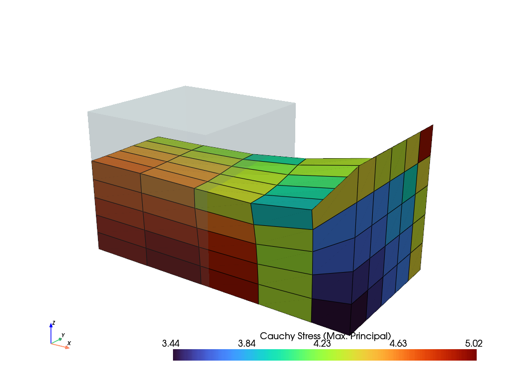
>>> solid.plot("Principal Values of Cauchy Stress").show()

Static Scene

Interactive Scene

References

See also

felupe.StateNearlyIncompressible: A State with internal cell-wise constant fields for (nearly) incompressible solid bodies.

class felupe.StateNearlyIncompressible(field)[source]#

Bases: object

A State with internal cell-wise constant dual fields for (nearly) incompressible solid bodies.

Notes

The internal fields \(p\) and \(\bar{J}\) are treated as state variables, directly derived from the displacement field. Hence, these dual fields are not exported to the global degrees of freedom.

Parameters:: field (FieldContainer) – A field container with the displacement field.

See also

felupe.SolidBodyNearlyIncompressible: A (nearly) incompressible solid body with methods for the assembly of sparse vectors/matrices.

integrate_shape_function_gradient(parallel=False, out=None)[source]#: Integrated sub-block matrix containing the shape-functions gradient w.r.t. the deformed coordinates \(\boldsymbol{K}_{\boldsymbol{u}p}\).

\[\int_V \delta \boldsymbol{F} : \frac{\partial J}{\partial \boldsymbol{F}} ~ dV\ \Delta p \longrightarrow \boldsymbol{K}_{\boldsymbol{u}p}\]

volume()[source]#: Return the cell volumes of the deformed configuration.

\[v = \int_V J ~ dV\]

class felupe.SolidBodyGravity(field, gravity=None, density=1.0)[source]#

Bases: object

A gravity (body) force on a solid body.

Parameters:

field (FieldContainer) – A field container with fields created on a boundary region.
gravity (ndarray or None, optional) – The prescribed values of gravity \(\boldsymbol{g}\) (default is None). If None, the gravity vector is set to zero (the dimension of the gravity vector is derived from the first field of the field container).
density (float, optional) – The density \(\rho\) of the solid body (default is 1.0).

Notes

\[\delta W_{ext} = \int_V \delta \boldsymbol{u} \cdot \rho \boldsymbol{g} \ dV\]

Examples

>>> import felupe as fem
>>>
>>> mesh = fem.Cube(n=6)
>>> region = fem.RegionHexahedron(mesh)
>>> field = fem.FieldContainer([fem.Field(region, dim=3)])
>>> boundaries = fem.dof.symmetry(field[0])
>>>
>>> umat = fem.NeoHooke(mu=1, bulk=2)
>>> solid = fem.SolidBody(umat, field)
>>> gravity = fem.SolidBodyGravity(field, density=1.0)
>>>
>>> table = fem.math.linsteps([0, 1], num=5, axis=0, axes=3)
>>> step = fem.Step(
...     items=[solid, gravity],
...     ramp={gravity: 2 * table},
...     boundaries=boundaries,
... )
>>>
>>> job = fem.Job(steps=[step]).evaluate()
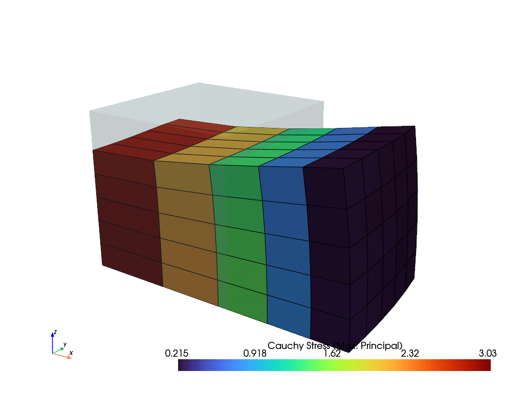
>>> solid.plot("Principal Values of Cauchy Stress").show()

Static Scene

Interactive Scene

update(gravity)[source]#

class felupe.SolidBodyPressure(field, pressure=None)[source]#

Bases: object

A hydrostatic pressure boundary on a solid body.

Parameters:

field (FieldContainer) – A field container with fields created on a boundary region.
pressure (float or ndarray or None, optional) – A scaling factor for the prescribed pressure \(p\) (default is None). If None, the pressure is set to zero.

Notes

\[\delta W_{ext} = \int_{\partial V} \delta \boldsymbol{u} \cdot p J \boldsymbol{F}^{-T} \ d\boldsymbol{A}\]

Examples

>>> import felupe as fem
>>>
>>> mesh = fem.Rectangle(n=6)
>>> region = fem.RegionQuad(mesh)
>>> field = fem.FieldContainer([fem.FieldAxisymmetric(region, dim=2)])
>>> boundaries = fem.dof.symmetry(field[0])
>>> umat = fem.NeoHooke(mu=1, bulk=2)
>>> solid = fem.SolidBody(umat, field)
>>>
>>> region_pressure = fem.RegionQuadBoundary(
...     mesh=mesh,
...     only_surface=True,  # select only faces on the outline
...     mask=mesh.points[:, 0] == 1,  # select a subset of faces on the surface
...     ensure_3d=True,  # requires True for axisymmetric/plane strain, otherwise False
... )
>>> field_boundary = fem.FieldContainer([fem.FieldAxisymmetric(region_pressure, dim=2)])
>>> pressure = fem.SolidBodyPressure(field=field_boundary)
>>>
>>> table = fem.math.linsteps([0, 1], num=5)
>>> step = fem.Step(
...     items=[solid, pressure], ramp={pressure: 1 * table}, boundaries=boundaries
... )
>>>
>>> job = fem.Job(steps=[step]).evaluate()
>>> solid.plot(
...     "Principal Values of Cauchy Stress", component=2, clim=[-1.01, -0.99]
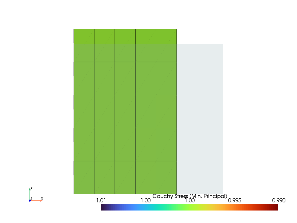
... ).show()

Static Scene

Interactive Scene

update(pressure)[source]#

class felupe.PointLoad(field, points, values=None, apply_on=0, axisymmetric=False)[source]#

Bases: object

A point load with methods for the assembly of sparse vectors/matrices.

update(values)[source]#

class felupe.Step(items, ramp=None, boundaries=None)[source]#

Bases: object

A Step with multiple substeps, subsequently depending on the solution of the previous substep.

Parameters:

items (list of SolidBody, SolidBodyNearlyIncompressible, SolidBodyPressure, SolidBodyGravity, PointLoad, MultiPointConstraint or MultiPointContact) – A list of items with methods for the assembly of sparse vectors/matrices.
ramp (dict, optional) – A dict with Boundary or item-keys which holds the array of values to ramp (default is None). If None, only one substep is evaluated.
boundaries (dict of Boundary, optional) – A dict with Boundary conditions (default is None).

Examples

>>> import felupe as fem
>>>
>>> mesh = fem.Cube(n=6)
>>> region = fem.RegionHexahedron(mesh)
>>> field = fem.FieldContainer([fem.Field(region, dim=3)])
>>>
>>> boundaries = fem.dof.symmetry(field[0])
>>> boundaries["clamped"] = fem.Boundary(field[0], fx=1, skip=(True, False, False))
>>> boundaries["move"] = fem.Boundary(field[0], fx=1, skip=(False, True, True))
>>>
>>> umat = fem.NeoHooke(mu=1, bulk=2)
>>> solid = fem.SolidBody(umat, field)
>>>
>>> move = fem.math.linsteps([0, 1], num=5)
>>> step = fem.Step(items=[solid], ramp={boundaries["move"]: move}, boundaries=boundaries)
>>>
>>> job = fem.Job(steps=[step]).evaluate()
>>> ax = solid.plot("Principal Values of Cauchy Stress").show()

Static Scene

Interactive Scene

generate(**kwargs)[source]#: Yield all generated substeps.

class felupe.Job(steps, callback=<function Job.<lambda>>, **kwargs)[source]#

Bases: object

A job with a list of steps and a method to evaluate them.

Parameters:

steps (list of Step) – A list with steps, where each step subsequently depends on the solution of the previous step.
callback (callable, optional) – A callable which is called after each completed substep. Function signature must be lambda stepnumber, substepnumber, substep, **kwargs: None, where substep is an instance of NewtonResult. The field container of the completed substep is available as substep.x. Default is callback=lambda stepnumber, substepnumber, substep, **kwargs: None.
**kwargs (dict, optional) – Optional keyword-arguments for the callback function.

steps#

A list with steps, where each step subsequently depends on the solution of the previous step.

Type:: list of Step

nsteps#

The number of steps.

Type:: int

callback#

A callable which is called after each completed substep. Function signature must be lambda stepnumber, substepnumber, substep: None, where substep is an instance of NewtonResult. THe field container of the completed substep is available as substep.x.

Type:: callable

timetrack#

A list with times at which the results are written to the XDMF result file.

Type:: list of int

fnorms#

List with norms of the objective function for each completed substep of each step. See also class:~felupe.tools.NewtonResult.

Type:: list of list of float

kwargs#

Optional keyword-arguments for the callback function.

Type:: dict

Examples

>>> import felupe as fem
>>>
>>> mesh = fem.Cube(n=6)
>>> region = fem.RegionHexahedron(mesh)
>>> field = fem.FieldContainer([fem.Field(region, dim=3)])
>>>
>>> boundaries = fem.dof.symmetry(field[0])
>>> boundaries["clamped"] = fem.Boundary(field[0], fx=1, skip=(True, False, False))
>>> boundaries["move"] = fem.Boundary(field[0], fx=1, skip=(False, True, True))
>>>
>>> umat = fem.NeoHooke(mu=1, bulk=2)
>>> solid = fem.SolidBody(umat, field)
>>>
>>> move = fem.math.linsteps([0, 1], num=5)
>>> step = fem.Step(items=[solid], ramp={boundaries["move"]: move}, boundaries=boundaries)
>>>
>>> job = fem.Job(steps=[step]).evaluate()
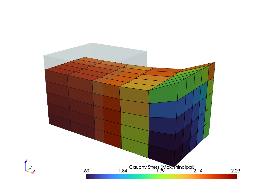
>>> solid.plot("Principal Values of Cauchy Stress").show()

Static Scene

Interactive Scene

See also

Step: A Step with multiple substeps, subsequently depending on the solution of the previous substep.
CharacteristicCurve: A job with a list of steps and a method to evaluate them. Force-displacement curve data is tracked during evaluation for a given Boundary.
tools.NewtonResult: A data class which represents the result found by Newton’s method.

evaluate(filename=None, mesh=None, point_data=None, cell_data=None, point_data_default=True, cell_data_default=True, verbose=None, parallel=False, **kwargs)[source]#

Evaluate the steps.

Parameters:

filename (str or None, optional) – The filename of the XDMF result file. Must include the file extension my_result.xdmf. If None, no result file is writte during evaluation. Default is None.
mesh (Mesh or None, optional) – A mesh which is used for the XDMF time series writer. If None, it is taken from the field of the first item of the first step if no keyword argument x0 is given. If None and x0=field, the mesh is taken from the x0 field container. Default is None.
point_data (dict or None, optional) – Additional dict of point-data for the meshio XDMF time series writer.
cell_data (dict or None, optional) – Additional dict of cell-data for the meshio XDMF time series writer.
point_data_default (bool, optional) – Flag to write default point-data to the XDMF result file. This includes "Displacement". Default is True.
cell_data_default (bool, optional) – Flag to write default cell-data to the XDMF result file. This includes "Principal Values of Logarithmic Strain", "Logarithmic Strain" and "Deformation Gradient". Default is True.
verbose (bool or int or None, optional) – Verbosity level to control how messages are printed during evaluation. If 1 or True and tqdm is installed, a progress bar is shown. If tqdm is missing or verbose is 2, more detailed text-based messages are printed. Default is None. If None, verbosity is set to True. If None and the environmental variable FELUPE_VERBOSE is set and its value is not true, then logging is turned off.
parallel (bool, optional) – Flag to use a threaded version of numpy.einsum() during assembly. Requires einsumt. This may add additional overhead to small-sized problems. Default is False.
**kwargs (dict) – Optional keyword arguments for generate(). If parallel=True, it is added as kwargs["parallel"] = True to the dict of additional keyword arguments. If x0 is present in kwargs.keys(), it is used as the mesh for the XDMF time series writer.

Returns:

The job object.

Return type:

Job

Notes

Requires meshio and h5py if filename is not None. Also requires tqdm for an interactive progress bar if verbose=True.

See also

Step: A Step with multiple substeps, subsequently depending on the solution of the previous substep.
CharacteristicCurve: A job with a list of steps and a method to evaluate them. Force-displacement curve data is tracked during evaluation for a given Boundary condition.
tools.NewtonResult: A data class which represents the result found by Newton’s method.

class felupe.CharacteristicCurve(steps, boundary, items=None, callback=<function CharacteristicCurve.<lambda>>, **kwargs)[source]#

Bases: Job

A job with a list of steps and a method to evaluate them. Force-displacement curve data is tracked during evaluation for a given Boundary by a built-in callback.

Parameters:

steps (list of Step) – A list with steps, where each step subsequently depends on the solution of the previous step.
items (list of SolidBody, SolidBodyNearlyIncompressible, SolidBodyPressure, SolidBodyGravity, PointLoad, MultiPointConstraint, MultiPointContact or None, optional) – A list of items with methods for the assembly of sparse vectors/matrices which are used to evaluate the sum of reaction forces. If None, the total reaction forces from the NewtonResult of the substep are used.
callback (callable, optional) – A callable which is called after each completed substep. Function signature must be lambda stepnumber, substepnumber, substep, **kwargs: None, where substep is an instance of NewtonResult. The field container of the completed substep is available as substep.x. Default is callback=lambda stepnumber, substepnumber, substep, **kwargs: None.
**kwargs (dict, optional) – Optional keyword-arguments for the callback function.

Examples

>>> import felupe as fem
>>>
>>> mesh = fem.Cube(n=6)
>>> region = fem.RegionHexahedron(mesh)
>>> field = fem.FieldContainer([fem.Field(region, dim=3)])
>>>
>>> boundaries = dict()
>>> boundaries["fixed"] = fem.Boundary(field[0], fx=0, skip=(False, False, False))
>>> boundaries["clamped"] = fem.Boundary(field[0], fx=1, skip=(True, False, False))
>>> boundaries["move"] = fem.Boundary(field[0], fx=1, skip=(False, True, True))
>>>
>>> umat = fem.NeoHooke(mu=1, bulk=2)
>>> solid = fem.SolidBody(umat, field)
>>>
>>> move = fem.math.linsteps([0, 1], num=5)
>>> step = fem.Step(items=[solid], ramp={boundaries["move"]: move}, boundaries=boundaries)
>>>
>>> job = fem.CharacteristicCurve(steps=[step], boundary=boundaries["move"]).evaluate()
>>> fig, ax = job.plot(
...    xlabel=r"Displacement $u_1$ in mm $\rightarrow$",
...    ylabel=r"Normal Force in $F_1$ in N $\rightarrow$",
...    marker="o",
... )

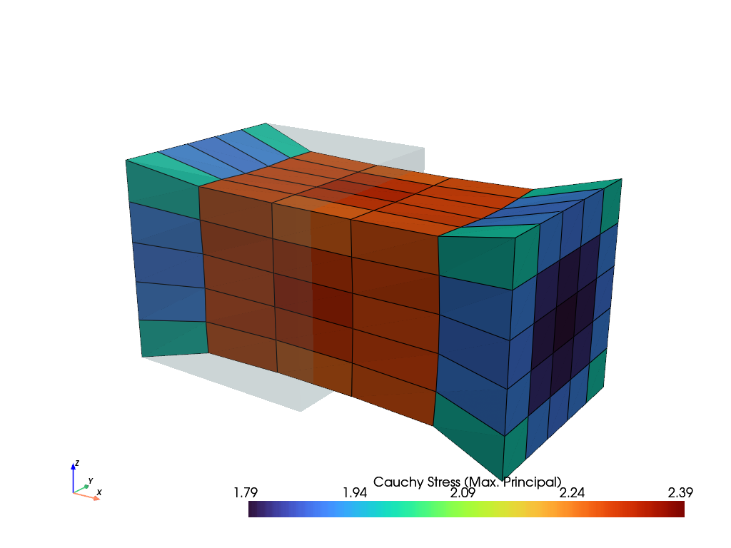
>>> solid.plot("Principal Values of Cauchy Stress").show()

Static Scene

Interactive Scene

See also

Step: A Step with multiple substeps, subsequently depending on the solution of the previous substep.
Job: A job with a list of steps and a method to evaluate them.
tools.NewtonResult: A data class which represents the result found by Newton’s method.

plot(x=None, y=None, xaxis=0, yaxis=0, xlabel=None, ylabel=None, xscale=1.0, yscale=1.0, xoffset=0.0, yoffset=0.0, gradient=False, swapaxes=False, ax=None, items=None, **kwargs)[source]#

Plot force-displacement characteristic curves on a pre-evaluated job, tracked on a given Boundary.

Parameters:

x (list of ndarray or None, optional) – A list with arrays of displacement data. If None, the displacement is taken from the first field of the field container from each completed substep. The displacement data is then taken from the first point of the tracked Boundary. Default is None.
y (list of ndarray or None, optional) – A list with arrays of reaction force data. If None, the force is taken from the NewtonResult of each completed substep. Default is None.
xaxis (int, optional) – The axis for the displacement data (default is 0).
yaxis (int, optional) – The axis for the reaction force data (default is 0).
xlabel (str or None, optional) – The label of the x-axis (default is None).
ylabel (str or None, optional) – The label of the y-axis (default is None).
xscale (float, optional) – A scaling factor for the displacement data (default is 1.0).
yscale (float, optional) – A scaling factor the reaction force data (default is 1.0).
xoffset (float, optional) – An offset for the displacement data (default is 0.0).
yoffset (float, optional) – An offset for the reaction force data (default is 0.0).
gradient (bool, optional) – A flag to plot the gradient of the y-data. Uses numpy.gradient(edge_order=2). The gradient data is set to np.nan for absolute values greater than the mean value plus two times the standard deviation. Default is False.
swapaxes (bool, optional) – A flag to flip the plot (x, y) to (y, x). Also changes the labels.
ax (matplotlib.axes.Axes) – An axes object where the plot is placed in.
items (slice, ndarray or None) – Indices or a range of data points to plot. If None, all data points are plotted (default is None).
**kwargs (dict) – Additional keyword arguments for plotting in ax.plot(**kwags).

Returns:

fig (matplotlib.figure.Figure) – The figure object where the plot is placed in.
ax (matplotlib.axes.Axes) – The axes object where the plot is placed in.

class felupe.MultiPointConstraint(field, points, centerpoint, skip=(False, False, False), multiplier=1000.0)[source]#

plot(plotter=None, color='black', **kwargs)[source]#

class felupe.MultiPointContact(field, points, centerpoint, skip=(False, False, False), multiplier=1000000.0)[source]#

plot(plotter=None, offset=0, show_edges=True, color='black', opacity=0.5, **kwargs)[source]#