Assembly

This module contains classes for the integration and assembly of (weak) integral forms into dense or sparse vectors and matrices. The integration algorithm switches automatically between general cartesion, plane strain or axisymmetric routines, dependent on the given fields.

Hint

IntegralForm is used in the Mechanics module (e.g. in a SolidBody) to integrate and/or assemble a constitutive material formulation and to provide an item for a Step or to use it in newtonrhapson() directly.

Core

Take arrays for some pre-defined weak-forms and integrate them into dense or assembly them into sparse vectors or matrices.

IntegralForm(fun, v, dV[, u, grad_v, grad_u])	Mixed-field integral form container with methods for integration and assembly.
assembly.IntegralFormCartesian(fun, v, dV[, ...])	Single-field integral form constructed by a function result fun, a test field v, differential volumes dV and optionally a trial field u.
assembly.IntegralFormAxisymmetric(fun, v, dV)	An Integral Form for axisymmetric fields.

Form Expressions

Define weak-form expressions on-the-fly for flexible and general form expressions.

Form(v[, u, dx, kwargs, parallel])

A linear or bilinear form object as function decorator on a weak-form with methods for integration and assembly of vectors or sparse matrices.

Create an item out of bilinear and linear weak-form expressions for a Step.

FormItem([bilinearform, linearform, sym, kwargs])

An item to be used in a felupe.Step with bilinear and optional linear form objects based on weak-forms with methods for integration and assembly of vectors / sparse matrices.

Detailed API Reference

class felupe.IntegralForm(fun, v, dV, u=None, grad_v=None, grad_u=None)

Mixed-field integral form container with methods for integration and assembly. It is constructed by a list of function results [fun, ...], a list of test fields [v, ...], differential volumes dV and optionally a list of trial fields [u, ...]. For the lists of fields, gradients may be passed by setting the respective list items in grad_v and grad_u to True.

Parameters:

• fun (list of array) – The list of pre-evaluated function arrays.

• v (FieldContainer) – The field container for the test fields.

• dV (array) – The differential volumes.

• u (FieldContainer, optional) – The field container for the trial fields. If a field container is passed, bilinear forms are created (default is None).

• grad_v (list of bool or None, optional) – List with flags to activate the gradients on the test fields v (default is None which enforces True for the first field and False for all following fields) .

• grad_u (list of bool or None, optional) – Flag to activate the gradient on the trial field u (default is None which enforces True for the first field and False for all following fields).

Notes

Linearform

A linear form is either defined by the dot product of a given (vector-valued) function \(\boldsymbol{f}\) and the (vector) field \(\boldsymbol{v}\)

\[L(\boldsymbol{v}) = \int_\Omega \boldsymbol{f} \cdot \boldsymbol{v} ~ dV\]

or by the double-dot product of a (matrix-valued) function \(\boldsymbol{f}\) and the gradient of the field values \(\boldsymbol{\nabla v}\).

\[L(\boldsymbol{v}) = \int_\Omega \boldsymbol{f} : \boldsymbol{\nabla v} ~ dV\]

Bilinearform

A bilinear form is either defined by the dot products of a given (matrix-valued) function \(\boldsymbol{f}\) and the (vector) fields \(\boldsymbol{v}\) and \(\boldsymbol{u}\)

\[a(\boldsymbol{v}, \boldsymbol{u}) = \int_\Omega \boldsymbol{v} \cdot \boldsymbol{f} \cdot \boldsymbol{u} ~ dV\]

or by the double-dot products of a (tensor-valued) function \(\boldsymbol{f}\) and the field values \(\boldsymbol{v}\) and \(\boldsymbol{u}\) or their gradients \(\boldsymbol{\nabla v}\) and \(\boldsymbol{\nabla u}\).

\[ \begin{align}\begin{aligned}a(\boldsymbol{v}, \boldsymbol{u}) &= \int_\Omega \boldsymbol{\nabla v} : \boldsymbol{f} \cdot \boldsymbol{u} ~ dV\\a(\boldsymbol{v}, \boldsymbol{u}) &= \int_\Omega \boldsymbol{v} \cdot \boldsymbol{f} : \boldsymbol{\nabla u} ~ dV\\a(\boldsymbol{v}, \boldsymbol{u}) &= \int_\Omega \boldsymbol{\nabla v} : \boldsymbol{f} : \boldsymbol{\nabla u} ~ dV\end{aligned}\end{align} \]

Examples

The stiffness matrix for a linear-elastic solid body on a cube out of hexahedrons is assembled as follows. First, the mesh, the region and the field objects are created.

>>> import felupe as fem
>>>
>>> mesh = fem.Cube(n=11)
>>> region = fem.RegionHexahedron(mesh)
>>> displacement = fem.Field(region, dim=3)
>>> field = fem.FieldContainer([displacement])

The (constant) fourth-order elasticity tensor for linear-elasticity is created with two trailing axes, one for each quadrature point and one for each cell. Due to the fact that the elasticity tensor is constant, broadcasting is used for the trailing axes.

\[\frac{\boldsymbol{\partial \sigma}}{\partial \boldsymbol{\varepsilon}} = 2 \mu \ \boldsymbol{I} \odot \boldsymbol{I} + \gamma \ \boldsymbol{I} \otimes \boldsymbol{I}\]

>>> import numpy as np
>>> from felupe.math import cdya, dya
>>>
>>> mu, lmbda = 1.0, 2.0
>>> I = np.eye(3).reshape(3, 3, 1, 1)
>>> dSdE = 2 * mu * cdya(I, I) + lmbda * dya(I, I)
>>> dSdE.shape
(3, 3, 3, 3, 1, 1)

The integral form object provides methods for cell-wise stiffness matrices via its integrate-method and the system stiffness matrix via the assembly-method.

\[\delta W_{int} = -\int_v \delta\boldsymbol{\varepsilon} : \frac{\boldsymbol{\partial \sigma}}{\partial \boldsymbol{\varepsilon}} : \boldsymbol{\varepsilon} ~ dv\]

\[ \begin{align}\begin{aligned}\delta\boldsymbol{\varepsilon} &= \text{sym}(\boldsymbol{\nabla v})\\\boldsymbol{\varepsilon} &= \text{sym}(\boldsymbol{\nabla u})\\\boldsymbol{\nabla v} &= \frac{\partial\boldsymbol{v}}{\partial\boldsymbol{x}}\\\boldsymbol{\nabla u} &= \frac{\partial\boldsymbol{u}}{\partial\boldsymbol{x}}\\\left( \frac{\partial v_i}{\partial x_j} \right)_{(qc)} &= \hat{v}_{ai} \left( \frac{\partial h_a}{\partial x_j} \right)_{(qc)}\end{aligned}\end{align} \]

\[\hat{K}_{aibk(c)} = \left( \frac{\partial h_a}{\partial x_J} \right)_{(qc)} \left( \frac{\partial \sigma_{ij}}{\partial \varepsilon_{kl}} \right)_{(qc)} \left( \frac{\partial h_b}{\partial x_L} \right)_{(qc)} ~ dv_{(qc)}\]

>>> form = fem.IntegralForm([dSdE], v=field, dV=region.dV, u=field)
>>> values = form.integrate(parallel=False)
>>> values[0].shape
(8, 3, 8, 3, 1000)

The cell-wise stiffness matrices are re-used to assemble the sparse system stiffness matrix. The parallel keyword argument enables a threaded assembly.

\[\Delta\delta W_{int} = -\hat{\boldsymbol{v}} : \hat{\boldsymbol{K}} : \hat{\boldsymbol{u}}\]

>>> K = form.assemble(values=values, parallel=False)
>>> K.shape
(3993, 3993)

See also

felupe.IntegralFormAxisymmetric

An Integral Form for axisymmetric fields.

felupe.IntegralFormCartesian

Single-field integral form.

felupe.Form

A weak-form expression decorator.

assemble(values=None, parallel=False, block=True, out=None)

integrate(parallel=False, out=None)

class felupe.assembly.IntegralFormCartesian(fun, v, dV, u=None, grad_v=False, grad_u=False)

Single-field integral form constructed by a function result fun, a test field v, differential volumes dV and optionally a trial field u. For both fields v and u gradients may be passed by setting grad_v and grad_u to True (default is False for both fields).

Parameters:

• fun (array) – The pre-evaluated function array.

• v (Field) – The test field.

• dV (array) – The differential volumes.

• u (Field, optional) – If a field is passed, a bilinear form is created (default is None).

• grad_v (bool, optional) – Flag to activate the gradient on the test field v (default is False).

• grad_u (bool, optional) – Flag to activate the gradient on the trial field u (default is False).

Notes

Linearform

A linear form is either defined by the dot product of a given (vector-valued) function \(\boldsymbol{f}\) and the (vector) field \(\boldsymbol{v}\)

\[L(\boldsymbol{v}) = \int_\Omega \boldsymbol{f} \cdot \boldsymbol{v} ~ dV\]

or by the double-dot product of a (matrix-valued) function \(\boldsymbol{F}\) and the gradient of the field values \(\boldsymbol{\nabla v}\).

\[L(\boldsymbol{v}) = \int_\Omega \boldsymbol{f} : \boldsymbol{\nabla v} ~ dV\]

Bilinearform

A bilinear form is either defined by the dot products of a given (matrix-valued) function \(\boldsymbol{f}\) and the (vector) fields \(\boldsymbol{v}\) and \(\boldsymbol{u}\)

\[a(\boldsymbol{v}, \boldsymbol{u}) = \int_\Omega \boldsymbol{v} \cdot \boldsymbol{f} \cdot \boldsymbol{u} ~ dV\]

or by the double-dot products of a (tensor-valued) function \(\boldsymbol{f}\) and the field values \(\boldsymbol{v}\) and \(\boldsymbol{u}\) or their gradients \(\boldsymbol{\nabla v}\) and \(\boldsymbol{\nabla u}\).

\[ \begin{align}\begin{aligned}a(\boldsymbol{v}, \boldsymbol{u}) &= \int_\Omega \boldsymbol{\nabla v} : \boldsymbol{f} \cdot \boldsymbol{u} ~ dV\\a(\boldsymbol{v}, \boldsymbol{u}) &= \int_\Omega \boldsymbol{v} \cdot \boldsymbol{f} : \boldsymbol{\nabla u} ~ dV\\a(\boldsymbol{v}, \boldsymbol{u}) &= \int_\Omega \boldsymbol{\nabla v} : \boldsymbol{f} : \boldsymbol{\nabla u} ~ dV\end{aligned}\end{align} \]

See also

felupe.IntegralForm

Mixed-field integral form container with methods for integration and assembly.

felupe.IntegralFormAxisymmetric

An Integral Form for axisymmetric fields.

assemble(values=None, parallel=False, out=None)

Assembly of sparse region vectors or matrices.

integrate(parallel=False, out=None)

Return evaluated (but not assembled) integrals.

class felupe.assembly.IntegralFormAxisymmetric(fun, v, dV, u=None, grad_v=True, grad_u=True)

An Integral Form for axisymmetric fields.

Notes

Axisymmetric scenarios are modeled with a 2D-mesh and consequently, a 2D element formulation. The rotation axis is chosen along the global X-axis \((X,Y,Z) \widehat{=} (Z,R,\varphi)\). The 3x3 deformation gradient consists of an in-plane 2x2 sub-matrix and one additional entry for the out-of-plane stretch which is equal to the ratio of deformed and undeformed radius.

\[\begin{split}\boldsymbol{F} = \begin{bmatrix} \boldsymbol{F}_{(2D)} & \boldsymbol{0} \\ \boldsymbol{0}^T & \frac{r}{R} \end{bmatrix}\end{split}\]

The variation of the deformation gradient consists of both in- and out-of-plane contributions.

\[\delta \boldsymbol{F}_{(2D)} = \delta \frac{ \partial \boldsymbol{u}}{\partial \boldsymbol{X} } \qquad \text{and} \qquad \delta \left(\frac{r}{R}\right) = \frac{\delta u_r}{R}\]

Again, the internal virtual work leads to two seperate terms.

\[-\delta W_{int} = \int_V \boldsymbol{P} : \delta \boldsymbol{F} \ dV = \int_V \boldsymbol{P}_{(2D)} : \delta \boldsymbol{F}_{(2D)} \ dV + \int_V \frac{P_{33}}{R} : \delta u_r \ dV\]

The differential volume is further expressed as a product of the differential in-plane area and the differential arc length. The arc length integral is finally pre-evaluated.

\[\int_V dV = \int_{\varphi=0}^{2\pi} \int_A R\ dA\ d\varphi = 2\pi \int_A R\ dA\]

Inserting the differential volume integral into the expression of internal virtual work, this leads to:

\[-\delta W_{int} = 2\pi \int_A \boldsymbol{P}_{(2D)} : \delta \boldsymbol{F}_{(2D)} \ R \ dA + 2\pi \int_A P_{33} : \delta u_r \ dA\]

A Linearization of the internal virtual work expression gives four terms.

\[ \begin{align}\begin{aligned}-\Delta \delta W_{int} &= \Delta_{(2D)} \delta_{(2D)} W_{int} + \Delta_{33} \delta_{(2D)} W_{int} + \Delta_{(2D)} \delta_{33} W_{int} + \Delta_{33} \delta_{33} W_{int}\\-\Delta_{(2D)} \delta_{(2D)} W_{int} &= 2\pi \int_A \delta \boldsymbol{F}_{(2D)} : \mathbb{A}_{(2D),(2D)} : \Delta \boldsymbol{F}_{(2D)} \ R \ dA\\-\Delta_{33} \delta_{(2D)} W_{int} &= 2\pi \int_A \delta \boldsymbol{F}_{(2D)} : \mathbb{A}_{(2D),33} : \Delta u_r \ dA\\-\Delta_{(2D)} \delta_{33} W_{int} &= 2\pi \int_A \delta u_r : \mathbb{A}_{33,(2D)} : \Delta \boldsymbol{F}_{(2D)} \ dA\\-\Delta_{33} \delta_{33} W_{int} &= 2\pi \int_A \delta u_r : \frac{\mathbb{A}_{33,33}}{R} : \Delta u_r \ dA\end{aligned}\end{align} \]

with

\[ \begin{align}\begin{aligned}\mathbb{A}_{(2D),(2D)} &= \frac{ \partial \psi}{\partial \boldsymbol{F}_{(2D)} \partial \boldsymbol{F}_{(2D)} }\\\mathbb{A}_{(2D),33} &= \frac{ \partial \psi}{\partial \boldsymbol{F}_{(2D)} \partial F^3_{\hphantom{3}3}} \left ( = \mathbb{A}_{33,(2D)} \right )\\\mathbb{A}_{33,33} &= \frac{\partial \psi}{F^3_{\hphantom{3}3} \partial F^3_{\hphantom{3}3}}\end{aligned}\end{align} \]

See also

felupe.IntegralForm

Mixed-field integral form container with methods for integration and assembly.

felupe.IntegralFormCartesian

Single-field integral form.

assemble(values=None, parallel=False, out=None)

Assembly of sparse region vectors or matrices.

integrate(parallel=False, out=None)

Return evaluated (but not assembled) integrals.

felupe.Form(v, u=None, dx=None, kwargs=None, parallel=False)

A linear or bilinear form object as function decorator on a weak-form with methods for integration and assembly of vectors or sparse matrices.

Parameters:

• v (FieldContainer) – A container for the v fields. May be updated during integration / assembly.

• u (FieldContainer) – A container for the u fields. May be updated during integration / assembly.

• dx (ndarray or None, optional) – Array with (numerical) differential volumes (default is None).

• kwargs (dict or None, optional) – Dictionary with initial optional weakform-keyword-arguments. May be updated during integration / assembly (default is None).

Returns:

A form object with methods for integration and assembly.

Return type:

FormExpression

Notes

Linear Form

\[L(v) = \int_\Omega f \cdot v \ dx\]

Bilinear Form

\[a(v, u) = \int_\Omega v \cdot f \cdot u \ dx\]

Examples

FElupe requires a pre-evaluated array for the definition of a bilinear felupe.IntegralForm object on interpolated field values or their gradients. While this has two benefits, namely a fast integration of the form is easy to code and the array may be computed in any programming language, sometimes numeric representations of analytic linear and bilinear form expressions may be easier in user-code and less error prone compared to the calculation of explicit second or fourth-order tensors. Therefore, FElupe provides a function decorator felupe.Form() as an easy-to-use high-level interface, similar to what scikit-fem offers. The felupe.Form() decorator handles a field container. The form class is similar, but not identical in its usage compared to felupe.IntegralForm. It requires a callable function (with optional arguments and keyword arguments) instead of a pre-computed array to be passed. The bilinear form of linear elasticity serves as a reference example for the demonstration on how to use this feature of FElupe. The stiffness matrix is assembled for a unit cube out of hexahedrons.

>>> import felupe as fem
>>>
>>> mesh = fem.Cube(n=6)
>>> region = fem.RegionHexahedron(mesh)
>>> displacement = fem.Field(region, dim=3)
>>> field = fem.FieldContainer([displacement])
>>>
>>> boundaries, loadcase = fem.dof.uniaxial(field, move=0.5, clamped=True)

The bilinear form of linear elasticity is defined as

\[a(v, u) = \int_\Omega 2 \mu \ \delta\boldsymbol{\varepsilon} : \boldsymbol{\varepsilon} + \lambda \ \text{tr}(\delta\boldsymbol{\varepsilon}) \ \text{tr}(\boldsymbol{\varepsilon}) \ dv\]

with

\[ \begin{align}\begin{aligned}\delta\boldsymbol{\varepsilon} &= \text{sym}(\text{grad}(\boldsymbol{v}))\\\boldsymbol{\varepsilon} &= \text{sym}(\text{grad}(\boldsymbol{u}))\end{aligned}\end{align} \]

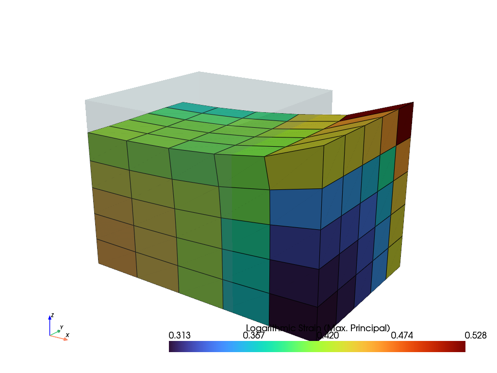
and implemented in FElupe closely to the analytic expression. The first two arguments for the callable weak-form function of a bilinear form are always arrays of field (gradients) (v, u) followed by arguments and keyword arguments. Optionally, the integration/assembly may be performed in parallel (threaded). Please note that this is only faster for relatively large systems. The weak-form function is decorated by felupe.Form() where the appropriate fields are linked to v and u along with the gradient flags for both fields. Arguments as well as keyword arguments of the weak-form may be defined inside the decorator or as part of the assembly arguments.

>>> from felupe.math import ddot, trace, sym, grad
>>>
>>> @fem.Form(v=field, u=field, kwargs={"μ": 1.0, "λ": 2.0})
... def bilinearform():
...     "A container for a bilinear form."
...
...     def linear_elasticity(v, u, μ, λ):
...         "Linear elasticity."
...
...         δε, ε = sym(grad(v)), sym(grad(u))
...         return 2 * μ * ddot(δε, ε) + λ * trace(δε) * trace(ε)
...
...     return [linear_elasticity,]
>>>
>>> stiffness_matrix = bilinearform.assemble(v=field, u=field, parallel=False)
>>>
>>> system = fem.solve.partition(
...     field, stiffness_matrix, dof1=loadcase["dof1"], dof0=loadcase["dof0"]
... )
>>> field += fem.solve.solve(*system, ext0=loadcase["ext0"])
>>> field.plot("Principal Values of Logarithmic Strain").show()

Static Scene

Interactive Scene

class felupe.FormItem(bilinearform=None, linearform=None, sym=False, kwargs=None)

An item to be used in a felupe.Step with bilinear and optional linear form objects based on weak-forms with methods for integration and assembly of vectors / sparse matrices.

Parameters:

• bilinearform (Form or None, optional) – A bilinear form object (default is None). If None, the resulting matrix will be filled with zeros.

• linearform (Form or None, optional) – A linear form object (default is None). If None, the resulting vector will be filled with zeros.

• sym (bool, optional) – Flag to active symmetric integration/assembly for bilinear forms (default is False).

• args (tuple or None, optional) – Tuple with initial optional weakform-arguments (default is None).

• kwargs (dict or None, optional) – Dictionary with initial optional weakform-keyword-arguments (default is None).

Examples

>>> import felupe as fem
>>> from felupe.math import ddot, sym, trace, grad
>>>
>>> mesh = fem.Cube(n=11)
>>> region = fem.RegionHexahedron(mesh)
>>> field = fem.FieldContainer([fem.Field(region, dim=3)])
>>> boundaries, loadcase = fem.dof.uniaxial(field, clamped=True)
>>>
>>> @fem.Form(v=field, u=field)
... def bilinearform():
...     def a(v, u, μ=1.0, λ=2.0):
...         δε, ε = sym(grad(v)), sym(grad(u))
...         return 2 * μ * ddot(δε, ε) + λ * trace(δε) * trace(ε)
...     return [a]
>>>
>>> item = fem.FormItem(bilinearform, linearform=None, sym=True)
>>> step = fem.Step(items=[item], boundaries=boundaries)
>>> job = fem.Job(steps=[step]).evaluate()

See also

felupe.Form

A function decorator for a linear- or bilinear-form object.

felupe.Step

A Step with multiple substeps.