Constitution#
This module provides constitutive material formulations.
Core frameworks and library with basic material models.
Advanced frameworks and material models with support for automatic differentiation.
Utilities to speed up repetitive & complicated tasks.
There are many different pre-defined constitutive material formulations available, including definitions for linear-elasticity, small-strain plasticity, hyperelasticity or pseudo-elasticity. The generation of user materials may be simplified when using frameworks for user-defined functions, like hyperelasticity (with automatic differentiation) or a small-strain based framework with state variables. However, the most general case is given by a framework with functions for the evaluation of stress and elasticity tensors in terms of the deformation gradient.
Constitutive Material Formulation
Base class for constitutive materials. |
|
|
A class-decorator for a constitutive material definition. |
Deformation Gradient-based Materials
|
A user-defined material definition with given functions for the (first Piola-Kirchhoff) stress tensor \(\boldsymbol{P}\), optional constraints on additional fields (e.g. \(p\) and \(J\)), updated state variables \(\boldsymbol{\zeta}\) as well as the according fourth-order elasticity tensor \(\mathbb{A}\) and the linearizations of the constraint equations. |
Detailed API Reference
- class felupe.ConstitutiveMaterial[source]#
Base class for constitutive materials.
A constitutive material definition, or so-called
umat(user material), is a class with methods for evaluating gradients and hessians of the strain energy density function with respect to the defined fields in the field container, where the gradient of the first (displacement) field is passed as the deformation gradient. For all following fields, the field values (no gradients) are provided. An attributex=[np.zeros(statevars_shape)]has to be added to the class to define the shape of optional state variables. For reasons of performance, FElupe passes the field gradients and values all at once, e.g. the deformation gradient is of shape(3, 3, q, c), whereqrefers to the number of quadrature points per cell andcto the number of cells. These last two axes are the so-called trailing axes. Math-functions from felupe.math all support the operation on trailing axes. The constitutive material definition class should be inherited fromConstitutiveMaterialin order to provide force-stretch curves for elementary deformations.Examples
Take this code-block as a template for a two-field \((\boldsymbol{u}, p)\) formulation with the old displacement gradient as a state variable:
import numpy as np
import felupe as fem

# math-functions which support trailing axes
from felupe.math import det, dya, identity, transpose, inv

class MyMaterialFormulation(fem.ConstitutiveMaterial):

    def __init__(self):
        # provide the shape of state variables without trailing axes
        # values are ignored - state variables are always initiated with zeros
        self.x = [np.zeros((3, 3))]

    def gradient(self, x):
        "Gradients of the strain energy density function."

        # extract variables
        F, p, statevars = x[0], x[1], x[-1]

        # user code
        dWdF = None  # first Piola-Kirchhoff stress tensor
        dWdp = None

        # update state variables
        # example: the displacement gradient
        statevars_new = F - identity(F)

        return [dWdF, dWdp, statevars_new]

    def hessian(self, x, **kwargs):
        "Hessians of the strain energy density function."

        # extract variables
        F, p, statevars = x[0], x[1], x[-1]

        # user code
        d2WdFdF = None  # fourth-order elasticity tensor
        d2WdFdp = None
        d2Wdpdp = None

        # upper-triangle items of the hessian
        return [d2WdFdF, d2WdFdp, d2Wdpdp]

umat = MyMaterialFormulation()
See also
felupe.constitutive_materialA decorator for a constitutive material definition.
- is_stable(x, hessian=None)[source]#
Return a boolean mask for stability of isotropic material model formulations.
At a given deformation gradient, a normal force is applied on each principal stretch direction. If the resulting incremental stretches are positive, the material model formulation is considered to be stable at the given deformation gradient.
- Parameters:
x (list of ndarray) – The list with input arguments. These contain the extracted fields of a
FieldContainer.hessian (ndarray or None, optional) – Second partial derivative of the strain energy density function w.r.t. the deformation gradient. Default is None.
- Returns:
Boolean mask of stability.
- Return type:
ndarray
Notes
Warning
This stability check will lead to a singular matrix for isotropic (hyperelastic) material model formulations without a volumetric part.
Examples
First, let’s check the stability of the Neo-Hookean material model formulation. The stability is evaluated on (valid) principal stretches of a biaxial deformation. All deformations are stable.
>>> import numpy as np
>>> import felupe as fem
>>>
>>> umat = fem.NeoHooke(mu=1.0, bulk=2.0)
>>> view = umat.view()
>>> λ = view.biaxial()[0]
>>>
>>> F = np.zeros((3, 3, 1, λ[0].size))
>>> for a in range(3):
...     F[a, a] = λ[a]
>>>
>>> umat.is_stable([F])
array([[ True,  True,  True,  True,  True,  True,  True,  True,  True,
         True,  True,  True,  True,  True,  True,  True]])
Now, let’s check the stability of the Mooney-Rivlin material model formulation. The stability is evaluated on (valid) principal stretches of a biaxial deformation. Biaxial deformations are only stable up to a longitudinal stretch of 1.35.
>>> import numpy as np
>>> import felupe as fem
>>> import felupe.constitution.tensortrax as mat
>>>
>>> umat = fem.Hyperelastic(
...     mat.models.hyperelastic.mooney_rivlin,
...     C10=0.25,
...     C01=0.25,
... ) & fem.Volumetric(bulk=5000)
>>> view = umat.view()
>>> λ = view.biaxial()[0]
>>>
>>> F = np.zeros((3, 3, 1, λ[0].size))
>>> for a in range(3):
...     F[a, a] = λ[a]
>>>
>>> umat.is_stable([F])
array([[ True,  True,  True,  True,  True,  True,  True,  True, False,
        False, False, False, False, False, False, False]])
- optimize(ux=None, ps=None, bx=None, incompressible=False, relative=False, **kwargs)[source]#
Optimize the material parameters by a least-squares fit on experimental stretch-stress data.
- Parameters:
ux (array of shape (2, ...) or None, optional) – Experimental uniaxial stretch and force-per-undeformed-area data (default is None).
ps (array of shape (2, ...) or None, optional) – Experimental planar-shear stretch and force-per-undeformed-area data (default is None).
bx (array of shape (2, ...) or None, optional) – Experimental biaxial stretch and force-per-undeformed-area data (default is None).
incompressible (bool, optional) – A flag to enforce incompressible deformations (default is False).
relative (bool, optional) – A flag to optimize relative instead of absolute residuals, i.e.
(predicted - observed) / observedinstead ofpredicted - observed(default is False).**kwargs (dict, optional) – Optional keyword arguments are passed to
scipy.optimize.least_squares().
- Returns:
ConstitutiveMaterial – A copy of the constitutive material with the optimized material parameters.
scipy.optimize.OptimizeResult – Represents the optimization result.
Notes
Warning
At least one load case, i.e. one of the arguments
ux,psorbxmust not beNone.Note
For JAX-based materials, double-precision is required to optimize material parameters.
import jax

jax.config.update("jax_enable_x64", True)
The vector of residuals is given in Eq. (3) in case of absolute residuals
(1)#\[ \begin{align}\begin{aligned}\begin{split}\boldsymbol{r} &= \begin{bmatrix} \boldsymbol{r}_\text{ux} \\ \boldsymbol{r}_\text{ps} \\ \boldsymbol{r}_\text{bx} \end{bmatrix}\end{split}\\r_\text{ux}(\lambda_i) &= P_\text{ux}(\lambda_i) - P_\text{ux, observed}(\lambda_i)\\r_\text{ps}(\lambda_i) &= P_\text{ps}(\lambda_i) - P_\text{ps, observed}(\lambda_i)\\r_\text{bx}(\lambda_i) &= P_\text{bx}(\lambda_i) - P_\text{bx, observed}(\lambda_i)\end{aligned}\end{align} \]and in Eq. (4) in case of relative residuals.
(2)#\[ \begin{align}\begin{aligned}\begin{split}\boldsymbol{r} &= \begin{bmatrix} \boldsymbol{r}_\text{ux} \\ \boldsymbol{r}_\text{ps} \\ \boldsymbol{r}_\text{bx} \end{bmatrix}\end{split}\\r_\text{ux}(\lambda_i) &= \frac{ P_\text{ux}(\lambda_i) - P_\text{ux, observed}(\lambda_i)}{ P_\text{ux, observed}(\lambda_i) }\\r_\text{ps}(\lambda_i) &= \frac{ P_\text{ps}(\lambda_i) - P_\text{ps, observed}(\lambda_i)}{ P_\text{ps, observed}(\lambda_i) }\\r_\text{bx}(\lambda_i) &= \frac{ P_\text{bx}(\lambda_i) - P_\text{bx, observed}(\lambda_i)}{ P_\text{bx, observed}(\lambda_i) }\end{aligned}\end{align} \]Examples
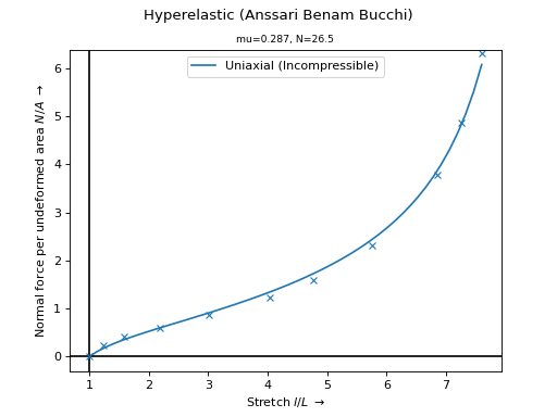
The
Anssari-Benam Bucchimaterial model formulation is best-fitted on Treloar’s uniaxial and biaxial tension data [1]_.>>> import numpy as np >>> import felupe as fem >>> >>> λ, P = np.array( ... [ ... [1.000, 0.00], ... [1.240, 2.30], ... [1.585, 4.16], ... [2.180, 6.00], ... [3.020, 8.80], ... [4.030, 12.5], ... [4.760, 16.2], ... [5.750, 23.6], ... [6.850, 38.5], ... [7.250, 49.6], ... [7.600, 64.4], ... ] ... ).T * np.array([[1.0], [0.0980665]]) >>> >>> umat = fem.Hyperelastic(fem.anssari_benam_bucchi) >>> umat_new, res = umat.optimize( ... ux=[λ, P], incompressible=True, relative=True ... ) >>> >>> ux = np.linspace(λ.min(), λ.max(), num=50) >>> ax = umat_new.plot(incompressible=True, ux=ux, bx=None, ps=None) >>> ax.plot(λ, P, "C0x")
See also
scipy.optimize.least_squaresSolve a nonlinear least-squares problem with bounds on the variables.
References
- plot(incompressible=False, **kwargs)[source]#
Return a plot with normal force per undeformed area vs. stretch curves for the elementary homogeneous deformations uniaxial tension/compression, planar shear and biaxial tension of a given isotropic material formulation.
- Parameters:
incompressible (bool, optional) – A flag to enforce views on incompressible deformations (default is False).
**kwargs (dict, optional) – Optional keyword-arguments for
ViewMaterialorViewMaterialIncompressible.
- Return type:
See also
felupe.ViewMaterialCreate views on normal force per undeformed area vs. stretch curves for the elementary homogeneous deformations uniaxial tension/compression, planar shear and biaxial tension of a given isotropic material formulation.
felupe.ViewMaterialIncompressibleCreate views on normal force per undeformed area vs. stretch curves for the elementary homogeneous incompressible deformations uniaxial tension/compression, planar shear and biaxial tension of a given isotropic material formulation.
- screenshot(filename='umat.png', incompressible=False, **kwargs)[source]#
Save a screenshot with normal force per undeformed area vs. stretch curves for the elementary homogeneous deformations uniaxial tension/compression, planar shear and biaxial tension of a given isotropic material formulation.
- Parameters:
filename (str, optional) – The filename of the screenshot (default is “umat.png”).
incompressible (bool, optional) – A flag to enforce views on incompressible deformations (default is False).
**kwargs (dict, optional) – Optional keyword-arguments for
ViewMaterialorViewMaterialIncompressible.
- Return type:
See also
felupe.ViewMaterialCreate views on normal force per undeformed area vs. stretch curves for the elementary homogeneous deformations uniaxial tension/compression, planar shear and biaxial tension of a given isotropic material formulation.
felupe.ViewMaterialIncompressibleCreate views on normal force per undeformed area vs. stretch curves for the elementary homogeneous incompressible deformations uniaxial tension/compression, planar shear and biaxial tension of a given isotropic material formulation.
- view(incompressible=False, **kwargs)[source]#
Create views on normal force per undeformed area vs. stretch curves for the elementary homogeneous deformations uniaxial tension/compression, planar shear and biaxial tension of a given isotropic material formulation.
- Parameters:
incompressible (bool, optional) – A flag to enforce views on incompressible deformations (default is False).
**kwargs (dict, optional) – Optional keyword-arguments for
ViewMaterialorViewMaterialIncompressible.
- Return type:
See also
felupe.ViewMaterialCreate views on normal force per undeformed area vs. stretch curves for the elementary homogeneous deformations uniaxial tension/compression, planar shear and biaxial tension of a given isotropic material formulation.
felupe.ViewMaterialIncompressibleCreate views on normal force per undeformed area vs. stretch curves for the elementary homogeneous incompressible deformations uniaxial tension/compression, planar shear and biaxial tension of a given isotropic material formulation.
- felupe.constitutive_material(Material, name=None)[source]#
A class-decorator for a constitutive material definition.
- Parameters:
Material (object) – A class with methods for the gradient and the hessian of the strain energy density function per unit undeformed volume w.r.t. the deformation gradient tensor.
name (str or None, optional) – The name of the derived class object. If None, the name is taken from
Material(default is None).
- Returns:
A derived class with multiple inheritance of
ConstitutiveMaterialandMaterial.- Return type:
Examples
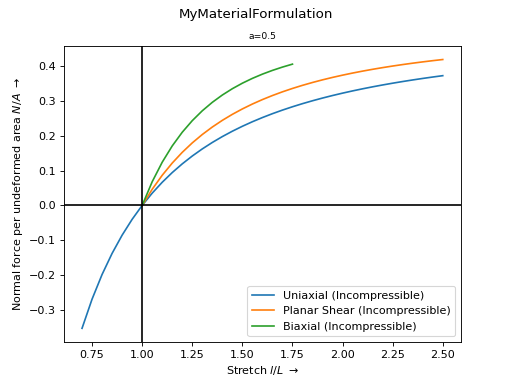
This example shows how to create a derived user material class to enable the methods from
ConstitutiveMaterialon any (external) material.>>> import felupe as fem >>> import numpy as np >>> >>> class MyMaterialFormulation: ... def __init__(self, a=5): ... self.x = [np.zeros((3, 3))] ... self.kwargs = {"a": a} ... ... def gradient(self, x): ... F, statevars = x[0], x[-1] ... dWdF = self.kwargs["a"] * np.eye(3).reshape(3, 3, 1, 1) ... return [dWdF, statevars] ... ... def hessian(self, x, **kwargs): ... F, statevars = x[0], x[-1] ... d2WdFdF = self.kwargs["a"] * np.zeros((3, 3, 3, 3, 1, 1)) ... return [d2WdFdF] >>> >>> MyMaterial = fem.constitutive_material(MyMaterialFormulation) >>> umat = MyMaterial(a=0.5) >>> ax = umat.plot(incompressible=True)
See also
felupe.ConstitutiveMaterialBase class for constitutive material formulations.
- class felupe.Material(stress, elasticity, nstatevars=0, **kwargs)[source]#
A user-defined material definition with given functions for the (first Piola-Kirchhoff) stress tensor \(\boldsymbol{P}\), optional constraints on additional fields (e.g. \(p\) and \(J\)), updated state variables \(\boldsymbol{\zeta}\) as well as the according fourth-order elasticity tensor \(\mathbb{A}\) and the linearizations of the constraint equations. Both functions take a list of the 3x3 deformation gradient \(\boldsymbol{F}\) and optional vector of state variables \(\boldsymbol{\zeta}_n\) as the first input argument. The stress-function must return the updated state variables \(\boldsymbol{\zeta}\).
- Parameters:
stress (callable) – A constitutive material definition which returns a list containing the (first Piola-Kirchhoff) stress tensor, optional additional constraints as well as the state variables. The state variables must always be included even if they are None. See template code-blocks for the required function signature.
elasticity (callable) – A constitutive material definition which returns a list containing the fourth- order elasticity tensor as the jacobian of the (first Piola-Kirchhoff) stress tensor w.r.t. the deformation gradient, optional linearizations of the additional constraints. The state variables must not be returned. See template code-blocks for the required function signature.
nstatevars (int, optional) – Number of internal state variable components (default is 0). State variable components must always be concatenated into a 1d-array.
Notes
Note
The first item in the list of the input arguments always contains the gradient of the (displacement) field \(\boldsymbol{u}\) w.r.t. the undeformed coordinates \(\boldsymbol{X}\). The identity matrix \(\boldsymbol{1}\) is added to this gradient, i.e. the first item of the list
xcontains the deformation gradient \(\boldsymbol{F} = \boldsymbol{1} + \frac{\partial \boldsymbol{u}}{\partial \boldsymbol{X}}\). All other fields are provided as interpolated values (no gradients evaluated).For \((\boldsymbol{u})\) single-field formulations, the callables for
stressandelasticitymust return the gradient and hessian of the strain energy density function \(\psi(\boldsymbol{F})\) w.r.t. the deformation gradient tensor \(\boldsymbol{F}\).\[\begin{split}\text{stress}(\boldsymbol{F}, \boldsymbol{\zeta}_n) = \begin{bmatrix} \frac{\partial \psi}{\partial \boldsymbol{F}} \\ \boldsymbol{\zeta} \end{bmatrix}\end{split}\]The callable for
elasticity(hessian) must not return the updated state variables.\[\text{elasticity}(\boldsymbol{F}, \boldsymbol{\zeta}_n) = \begin{bmatrix} \frac{\partial^2 \psi}{\partial \boldsymbol{F}\ \partial \boldsymbol{F}} \end{bmatrix}\]Take this code-block as template:
def stress(x, **kwargs):
    "First Piola-Kirchhoff stress tensor."

    # extract variables
    F, statevars = x[0], x[-1]

    # user code for (first Piola-Kirchhoff) stress tensor
    P = None

    # update state variables
    statevars_new = None

    return [P, statevars_new]

def elasticity(x, **kwargs):
    "Fourth-order elasticity tensor."

    # extract variables
    F, statevars = x[0], x[-1]

    # user code for fourth-order elasticity tensor
    # according to the (first Piola-Kirchhoff) stress tensor
    dPdF = None

    return [dPdF]

umat = Material(stress, elasticity, **kwargs)
For \((\boldsymbol{u}, p, J)\) mixed-field formulations, the callables for
stressandelasticitymust return the gradients and hessians of the (augmented) strain energy density function w.r.t. the deformation gradient and the other fields.\[\begin{split}\text{stress}(\boldsymbol{F}, p, J, \boldsymbol{\zeta}_n) = \begin{bmatrix} \frac{\partial \psi}{\partial \boldsymbol{F}} \\ \frac{\partial \psi}{\partial p} \\ \frac{\partial \psi}{\partial J} \\ \boldsymbol{\zeta} \end{bmatrix}\end{split}\]For the hessians, the upper-triangle blocks have to be provided.
\[\begin{split}\text{elasticity}(\boldsymbol{F}, p, J, \boldsymbol{\zeta}_n) = \begin{bmatrix} \frac{\partial^2 \psi}{\partial \boldsymbol{F}\ \partial \boldsymbol{F}} \\ \frac{\partial^2 \psi}{\partial \boldsymbol{F}\ \partial p} \\ \frac{\partial^2 \psi}{\partial \boldsymbol{F}\ \partial J} \\ \frac{\partial^2 \psi}{\partial p\ \partial p} \\ \frac{\partial^2 \psi}{\partial p\ \partial J} \\ \frac{\partial^2 \psi}{\partial J\ \partial J} \end{bmatrix}\end{split}\]For \((\boldsymbol{u}, p, J)\) mixed-field formulations, take this code-block as template:
def gradient(x, **kwargs):
    "Gradients of the strain energy density function."

    # extract variables
    F, p, J, statevars = x[0], x[1], x[2], x[-1]

    # user code
    dWdF = None  # first Piola-Kirchhoff stress tensor
    dWdp = None
    dWdJ = None

    # update state variables
    statevars_new = None

    return [dWdF, dWdp, dWdJ, statevars_new]

def hessian(x, **kwargs):
    "Hessians of the strain energy density function."

    # extract variables
    F, p, J, statevars = x[0], x[1], x[2], x[-1]

    # user code
    d2WdFdF = None  # fourth-order elasticity tensor
    d2WdFdp = None
    d2WdFdJ = None
    d2Wdpdp = None
    d2WdpdJ = None
    d2WdJdJ = None

    # upper-triangle items of the hessian
    return [d2WdFdF, d2WdFdp, d2WdFdJ, d2Wdpdp, d2WdpdJ, d2WdJdJ]

umat = Material(gradient, hessian, **kwargs)
Examples
The compressible isotropic hyperelastic Neo-Hookean material formulation is given by the strain energy density function
\[\psi(\boldsymbol{C}) = \frac{\mu}{2} \text{tr}(\boldsymbol{C}) - \mu \ln(J) + \frac{\lambda}{2} \ln(J)^2\]with the determinant of the deformation gradient and the right Cauchy Green deformation tensor.
\[ \begin{align}\begin{aligned}J &= \text{det}(\boldsymbol{F})\\C &= \boldsymbol{F}^T\ \boldsymbol{F}\end{aligned}\end{align} \]The first Piola-Kirchhoff stress tensor is evaluated as the gradient of the strain energy density function.
\[ \begin{align}\begin{aligned}\boldsymbol{P} &= \frac{\partial \psi}{\partial \boldsymbol{F}}\\\boldsymbol{P} &= \mu \left( \boldsymbol{F} - \boldsymbol{F}^{-T} \right) + \lambda \ln(J) \boldsymbol{F}^{-T}\end{aligned}\end{align} \]The hessian of the strain energy density function enables the corresponding elasticity tensor.
\[ \begin{align}\begin{aligned}\mathbb{A} &= \frac{\partial^2 \psi}{\partial \boldsymbol{F}\ \partial \boldsymbol{F}}\\\mathbb{A} &= \mu \boldsymbol{I} \overset{ik}{\otimes} \boldsymbol{I} + \left(\mu - \lambda \ln(J) \right) \boldsymbol{F}^{-T} \overset{il}{\otimes} \boldsymbol{F}^{-T} + \lambda \boldsymbol{F}^{-T} {\otimes} \boldsymbol{F}^{-T}\end{aligned}\end{align} \]>>> import numpy as np >>> import felupe as fem >>> >>> from felupe.math import ( ... cdya_ik, ... cdya_il, ... det, ... dya, ... identity, ... inv, ... transpose ... ) >>> >>> def stress(x, mu, lmbda): ... F, statevars = x[0], x[-1] ... J = det(F) ... lnJ = np.log(J) ... iFT = transpose(inv(F, J)) ... dWdF = mu * (F - iFT) + lmbda * lnJ * iFT ... return [dWdF, statevars] >>> >>> def elasticity(x, mu, lmbda): ... F = x[0] ... J = det(F) ... iFT = transpose(inv(F, J)) ... eye = identity(F) ... return [ ... mu * cdya_ik(eye, eye) + lmbda * dya(iFT, iFT) + ... (mu - lmbda * np.log(J)) * cdya_il(iFT, iFT) ... ] >>>
The material formulation is tested in a minimal example of non-homogeneous uniaxial tension.
>>> mesh = fem.Cube(n=3)
>>> region = fem.RegionHexahedron(mesh)
>>> field = fem.FieldContainer([fem.Field(region, dim=3)])
>>>
>>> umat = fem.Material(stress, elasticity, mu=1.0, lmbda=2.0)
>>> solid = fem.SolidBodyNearlyIncompressible(umat, field, bulk=5000)
>>>
>>> boundaries = fem.dof.uniaxial(
...     field, clamped=True, move=0.5, return_loadcase=False
... )
>>>
>>> step = fem.Step(items=[solid], boundaries=boundaries)
>>> job = fem.Job(steps=[step]).evaluate()
See also
felupe.NeoHookeCompressibleNearly-incompressible isotropic hyperelastic Neo-Hookean material formulation.
- copy()#
Return a deep-copy of the constitutive material.
- gradient(x)[source]#
Return the evaluated gradient of the strain energy density function.
- Parameters:
x (list of ndarray) – The list with input arguments. These contain the extracted fields of a
FieldContaineralong with the old vector of state variables,[*field.extract(), statevars_old].- Returns:
A list with the evaluated gradient(s) of the strain energy density function and the updated vector of state variables.
- Return type:
list of ndarray
- hessian(x)[source]#
Return the evaluated upper-triangle components of the hessian(s) of the strain energy density function.
- Parameters:
x (list of ndarray) – The list with input arguments. These contain the extracted fields of a
FieldContaineralong with the old vector of state variables,[*field.extract(), statevars_old].- Returns:
A list with the evaluated upper-triangle components of the hessian(s) of the strain energy density function.
- Return type:
list of ndarray
- is_stable(x, hessian=None)#
Return a boolean mask for stability of isotropic material model formulations.
At a given deformation gradient, a normal force is applied on each principal stretch direction. If the resulting incremental stretches are positive, the material model formulation is considered to be stable at the given deformation gradient.
- Parameters:
x (list of ndarray) – The list with input arguments. These contain the extracted fields of a
FieldContainer.hessian (ndarray or None, optional) – Second partial derivative of the strain energy density function w.r.t. the deformation gradient. Default is None.
- Returns:
Boolean mask of stability.
- Return type:
ndarray
Notes
Warning
This stability check will lead to a singular matrix for isotropic (hyperelastic) material model formulations without a volumetric part.
Examples
First, let’s check the stability of the Neo-Hookean material model formulation. The stability is evaluated on (valid) principal stretches of a biaxial deformation. All deformations are stable.
>>> import numpy as np
>>> import felupe as fem
>>>
>>> umat = fem.NeoHooke(mu=1.0, bulk=2.0)
>>> view = umat.view()
>>> λ = view.biaxial()[0]
>>>
>>> F = np.zeros((3, 3, 1, λ[0].size))
>>> for a in range(3):
...     F[a, a] = λ[a]
>>>
>>> umat.is_stable([F])
array([[ True,  True,  True,  True,  True,  True,  True,  True,  True,
         True,  True,  True,  True,  True,  True,  True]])
Now, let’s check the stability of the Mooney-Rivlin material model formulation. The stability is evaluated on (valid) principal stretches of a biaxial deformation. Biaxial deformations are only stable up to a longitudinal stretch of 1.35.
>>> import numpy as np
>>> import felupe as fem
>>> import felupe.constitution.tensortrax as mat
>>>
>>> umat = fem.Hyperelastic(
...     mat.models.hyperelastic.mooney_rivlin,
...     C10=0.25,
...     C01=0.25,
... ) & fem.Volumetric(bulk=5000)
>>> view = umat.view()
>>> λ = view.biaxial()[0]
>>>
>>> F = np.zeros((3, 3, 1, λ[0].size))
>>> for a in range(3):
...     F[a, a] = λ[a]
>>>
>>> umat.is_stable([F])
array([[ True,  True,  True,  True,  True,  True,  True,  True, False,
        False, False, False, False, False, False, False]])
- optimize(ux=None, ps=None, bx=None, incompressible=False, relative=False, **kwargs)#
Optimize the material parameters by a least-squares fit on experimental stretch-stress data.
- Parameters:
ux (array of shape (2, ...) or None, optional) – Experimental uniaxial stretch and force-per-undeformed-area data (default is None).
ps (array of shape (2, ...) or None, optional) – Experimental planar-shear stretch and force-per-undeformed-area data (default is None).
bx (array of shape (2, ...) or None, optional) – Experimental biaxial stretch and force-per-undeformed-area data (default is None).
incompressible (bool, optional) – A flag to enforce incompressible deformations (default is False).
relative (bool, optional) – A flag to optimize relative instead of absolute residuals, i.e.
(predicted - observed) / observedinstead ofpredicted - observed(default is False).**kwargs (dict, optional) – Optional keyword arguments are passed to
scipy.optimize.least_squares().
- Returns:
ConstitutiveMaterial – A copy of the constitutive material with the optimized material parameters.
scipy.optimize.OptimizeResult – Represents the optimization result.
Notes
Warning
At least one load case, i.e. one of the arguments
ux,psorbxmust not beNone.Note
For JAX-based materials, double-precision is required to optimize material parameters.
import jax

jax.config.update("jax_enable_x64", True)
The vector of residuals is given in Eq. (3) in case of absolute residuals
(3)#\[ \begin{align}\begin{aligned}\begin{split}\boldsymbol{r} &= \begin{bmatrix} \boldsymbol{r}_\text{ux} \\ \boldsymbol{r}_\text{ps} \\ \boldsymbol{r}_\text{bx} \end{bmatrix}\end{split}\\r_\text{ux}(\lambda_i) &= P_\text{ux}(\lambda_i) - P_\text{ux, observed}(\lambda_i)\\r_\text{ps}(\lambda_i) &= P_\text{ps}(\lambda_i) - P_\text{ps, observed}(\lambda_i)\\r_\text{bx}(\lambda_i) &= P_\text{bx}(\lambda_i) - P_\text{bx, observed}(\lambda_i)\end{aligned}\end{align} \]and in Eq. (4) in case of relative residuals.
(4)#\[ \begin{align}\begin{aligned}\begin{split}\boldsymbol{r} &= \begin{bmatrix} \boldsymbol{r}_\text{ux} \\ \boldsymbol{r}_\text{ps} \\ \boldsymbol{r}_\text{bx} \end{bmatrix}\end{split}\\r_\text{ux}(\lambda_i) &= \frac{ P_\text{ux}(\lambda_i) - P_\text{ux, observed}(\lambda_i)}{ P_\text{ux, observed}(\lambda_i) }\\r_\text{ps}(\lambda_i) &= \frac{ P_\text{ps}(\lambda_i) - P_\text{ps, observed}(\lambda_i)}{ P_\text{ps, observed}(\lambda_i) }\\r_\text{bx}(\lambda_i) &= \frac{ P_\text{bx}(\lambda_i) - P_\text{bx, observed}(\lambda_i)}{ P_\text{bx, observed}(\lambda_i) }\end{aligned}\end{align} \]Examples
The
Anssari-Benam Bucchimaterial model formulation is best-fitted on Treloar’s uniaxial and biaxial tension data [1]_.>>> import numpy as np >>> import felupe as fem >>> >>> λ, P = np.array( ... [ ... [1.000, 0.00], ... [1.240, 2.30], ... [1.585, 4.16], ... [2.180, 6.00], ... [3.020, 8.80], ... [4.030, 12.5], ... [4.760, 16.2], ... [5.750, 23.6], ... [6.850, 38.5], ... [7.250, 49.6], ... [7.600, 64.4], ... ] ... ).T * np.array([[1.0], [0.0980665]]) >>> >>> umat = fem.Hyperelastic(fem.anssari_benam_bucchi) >>> umat_new, res = umat.optimize( ... ux=[λ, P], incompressible=True, relative=True ... ) >>> >>> ux = np.linspace(λ.min(), λ.max(), num=50) >>> ax = umat_new.plot(incompressible=True, ux=ux, bx=None, ps=None) >>> ax.plot(λ, P, "C0x")

See also
scipy.optimize.least_squaresSolve a nonlinear least-squares problem with bounds on the variables.
References
- plot(incompressible=False, **kwargs)#
Return a plot with normal force per undeformed area vs. stretch curves for the elementary homogeneous deformations uniaxial tension/compression, planar shear and biaxial tension of a given isotropic material formulation.
- Parameters:
incompressible (bool, optional) – A flag to enforce views on incompressible deformations (default is False).
**kwargs (dict, optional) – Optional keyword-arguments for
ViewMaterialorViewMaterialIncompressible.
- Return type:
See also
felupe.ViewMaterialCreate views on normal force per undeformed area vs. stretch curves for the elementary homogeneous deformations uniaxial tension/compression, planar shear and biaxial tension of a given isotropic material formulation.
felupe.ViewMaterialIncompressibleCreate views on normal force per undeformed area vs. stretch curves for the elementary homogeneous incompressible deformations uniaxial tension/compression, planar shear and biaxial tension of a given isotropic material formulation.
- screenshot(filename='umat.png', incompressible=False, **kwargs)#
Save a screenshot with normal force per undeformed area vs. stretch curves for the elementary homogeneous deformations uniaxial tension/compression, planar shear and biaxial tension of a given isotropic material formulation.
- Parameters:
filename (str, optional) – The filename of the screenshot (default is “umat.png”).
incompressible (bool, optional) – A flag to enforce views on incompressible deformations (default is False).
**kwargs (dict, optional) – Optional keyword-arguments for
ViewMaterialorViewMaterialIncompressible.
- Return type:
See also
felupe.ViewMaterialCreate views on normal force per undeformed area vs. stretch curves for the elementary homogeneous deformations uniaxial tension/compression, planar shear and biaxial tension of a given isotropic material formulation.
felupe.ViewMaterialIncompressibleCreate views on normal force per undeformed area vs. stretch curves for the elementary homogeneous incompressible deformations uniaxial tension/compression, planar shear and biaxial tension of a given isotropic material formulation.
- view(incompressible=False, **kwargs)#
Create views on normal force per undeformed area vs. stretch curves for the elementary homogeneous deformations uniaxial tension/compression, planar shear and biaxial tension of a given isotropic material formulation.
- Parameters:
incompressible (bool, optional) – A flag to enforce views on incompressible deformations (default is False).
**kwargs (dict, optional) – Optional keyword-arguments for
ViewMaterialorViewMaterialIncompressible.
- Return type:
See also
felupe.ViewMaterialCreate views on normal force per undeformed area vs. stretch curves for the elementary homogeneous deformations uniaxial tension/compression, planar shear and biaxial tension of a given isotropic material formulation.
felupe.ViewMaterialIncompressibleCreate views on normal force per undeformed area vs. stretch curves for the elementary homogeneous incompressible deformations uniaxial tension/compression, planar shear and biaxial tension of a given isotropic material formulation.