Mixed-Field Problems

FElupe supports mixed-field formulations in a similar way it can handle (default) single-field formulations. The definition of a mixed-field formulation is shown for the hydrostatic-volumetric selective three-field-variation with independend fields for displacements \(\boldsymbol{u}\), pressure \(p\) and volume ratio \(J\). The total potential energy for nearly-incompressible hyperelasticity is formulated with a determinant-modified deformation gradient. The built-in Neo-Hookean material model is used as an argument of ThreeFieldVariation for mixed-field problems.

import felupe as fem

neohooke = fem.constitution.NeoHooke(mu=1.0, bulk=5000.0)
umat = fem.constitution.ThreeFieldVariation(neohooke)

Next, let’s create a meshed cube for a Hood-Taylor element formulation. The family of Hood-Taylor elements have a pressure field which is one order lower than the displacement field. A Hood-Taylor Q2/P1 hexahedron element formulation is created, where a tri-quadratic continuous (Lagrange) 27-point per cell displacement formulation is used in combination with discontinuous (tetra) 4-point per cell formulations for the pressure and volume ratio fields. The mesh of the cube is converted to a tri-quadratic mesh for the displacement field. The tetra regions for the pressure and the volume ratio are created on a dual (disconnected) mesh for the generation of the discontinuous fields.

mesh  = fem.Cube(n=5)
mesh_q2 = mesh.convert(
    order=2,
    calc_points=True,
    calc_midfaces=True,
    calc_midvolumes=True
)

region_q2 = fem.RegionTriQuadraticHexahedron(mesh_q2)
region_p1 = fem.RegionTetra(
    mesh=mesh.dual(points_per_cell=4),
    quadrature=region_q2.quadrature,
    grad=False
)

displacement = fem.Field(region_q2,  dim=3)
pressure     = fem.Field(region_p1, dim=1)
volumeratio  = fem.Field(region_p1, dim=1, values=1.0)

field = fem.FieldContainer(fields=[displacement, pressure, volumeratio])
solid = fem.SolidBody(umat=umat, field=field)

Boundary conditions are enforced on the displacement field. For the pre-defined loadcases like the clamped uniaxial compression, the boundaries are automatically applied on the first field.

boundaries, loadcase = fem.dof.uniaxial(field, clamped=True)

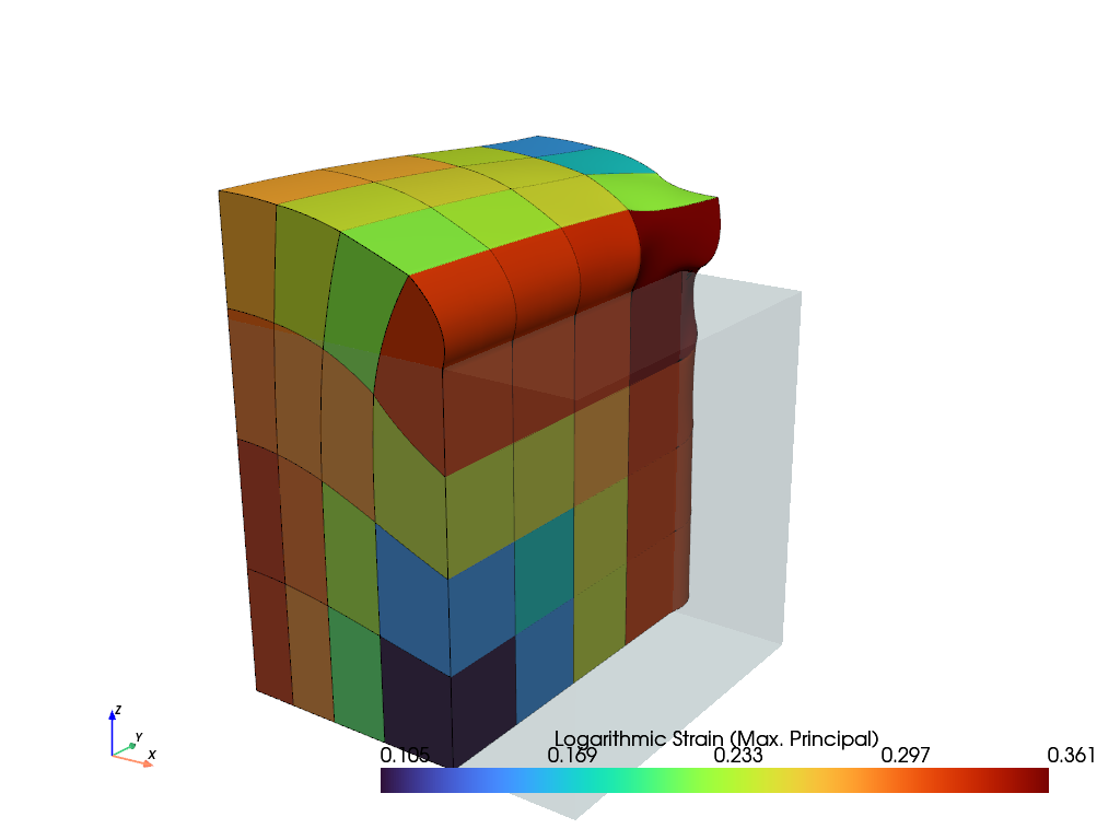
The Step and Job definitions are identical to ones used with single field formulations. The deformed cube is finally visualized by PyVista. The cell-based means of the maximum principal values of the logarithmic strain tensor are shown.

step = fem.Step(
    items=[solid],
    ramp={boundaries["move"]: fem.math.linsteps([0, -0.35], num=10)},
    boundaries=boundaries
)
job = fem.CharacteristicCurve(steps=[step], boundary=boundaries["move"])
job.evaluate(filename="result.xdmf")

field.plot("Principal Values of Logarithmic Strain", nonlinear_subdivision=4).show()