Multiple Solid Bodies

This section demonstrates how to set up a problem with two regions, each associated to a seperated solid body. Different element formulations are used for the solid bodies.

import felupe as fem

inner = fem.Rectangle(a=(-1, -1), b=(1, 1), n=(5, 5)).triangulate()

lower = fem.Rectangle(a=(-3, -3), b=(3, -1), n=(13, 5))
upper = fem.Rectangle(a=(-3, 1), b=(3, 3), n=(13, 5))
left = fem.Rectangle(a=(-3, -1), b=(-1, 1), n=(5, 5))
right = fem.Rectangle(a=(1, -1), b=(3, 1), n=(5, 5))

outer = fem.MeshContainer([lower, upper, left, right], merge=True).stack()

container = fem.MeshContainer([inner, outer], merge=True)

A top-level (vertex) field, which contains all the unknowns, is required for the definition of the boundary conditions as well as for the evaluation of the job.

Note

Ensure to init the mesh container with merge=True, otherwise the points-array of the container will be empty.

container = fem.MeshContainer([inner, outer], merge=True)
field = fem.Field.from_mesh_container(container).as_container()

field.plot(plotter=container.plot(), point_size=15, color="red").show()

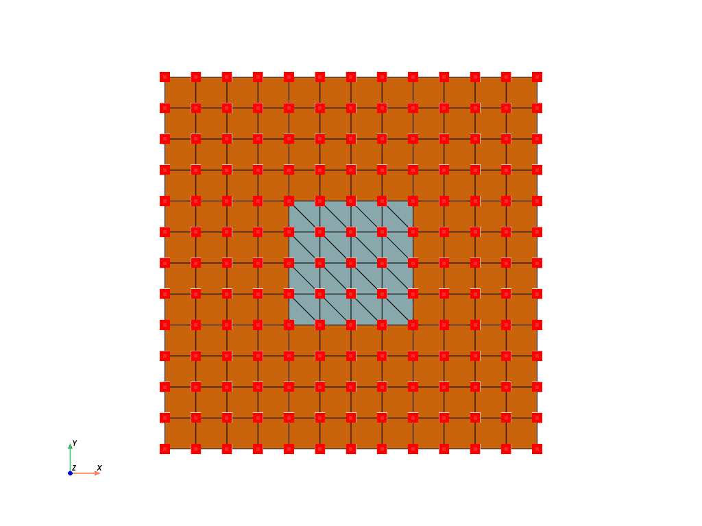
The sub-meshes are available in the global mesh container, on which the sub-fields are created.

regions = [
    fem.RegionTriangle(container.meshes[0]),
    fem.RegionQuad(container.meshes[1]),
]
fields = [
    fem.FieldContainer([fem.FieldPlaneStrain(regions[0], dim=2)]),
    fem.FieldContainer([fem.FieldPlaneStrain(regions[1], dim=2)]),
]

The displacement boundaries are created on the top-level field.

boundaries = dict(
    fixed=fem.Boundary(field[0], fx=field.region.mesh.x.min()),
    move=fem.Boundary(field[0], fx=field.region.mesh.x.max()),
)

The rubber is associated to a Neo-Hookean material formulation whereas the steel is modeled by a linear elastic material formulation. Due to the large rotation, its large-strain formulation is required. For each material a solid body is created.

# two material model formulations
linear_elastic = fem.LinearElasticLargeStrain(E=100, nu=0.3)
neo_hooke = fem.NeoHooke(mu=1, bulk=1)

# the solid bodies
fiber = fem.SolidBody(umat=linear_elastic, field=fields[0])
matrix = fem.SolidBody(umat=neo_hooke, field=fields[1])

A step is created and further added to a job. The global field must be passed as the x0 argument during the evaluation of the job. Internally, all field values are linked automatically, i.e. they share their values array.

# prepare a step with substeps
move = fem.math.linsteps([0, 3], num=10)
step = fem.Step(
    items=[matrix, fiber],
    ramp={boundaries["move"]: move},
    boundaries=boundaries,
)

# take care of the x0-argument
job = fem.Job(steps=[step])
job.evaluate(x0=field)

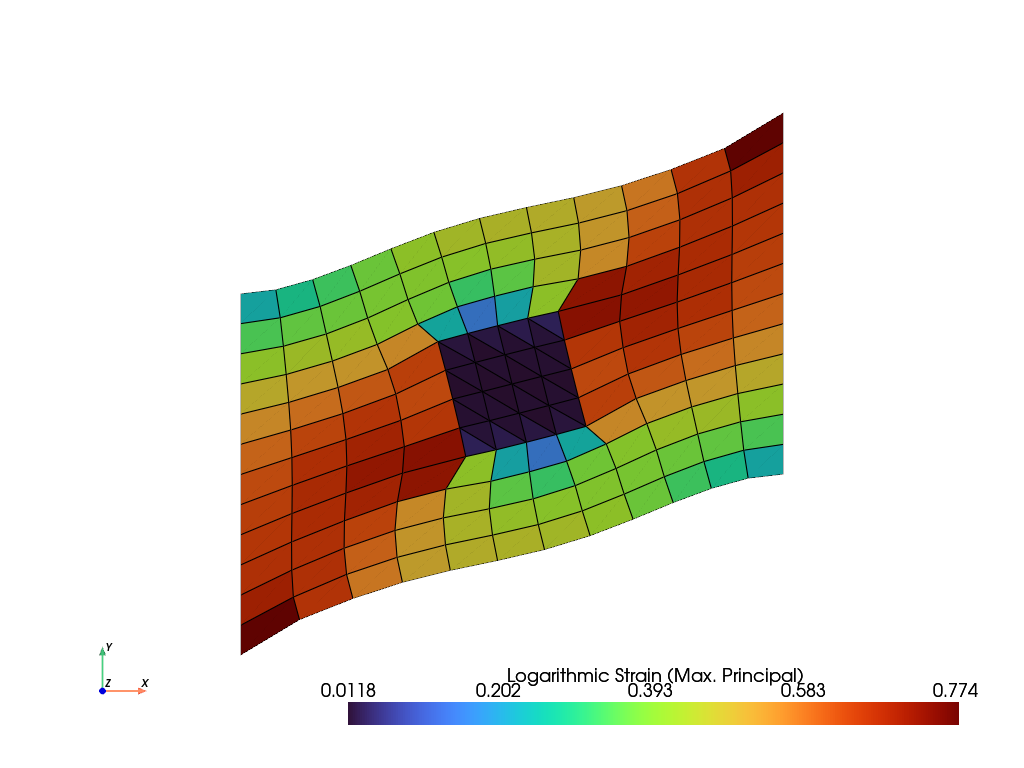
fields[1].plot(
    "Principal Values of Logarithmic Strain",
    show_undeformed=False,
    plotter=fields[0].plot(
        "Principal Values of Logarithmic Strain", show_undeformed=False
    ),
).show()