Generate Meshes#
FElupe provides a simple mesh generation module mesh. A Mesh instance contains essentially two arrays: one with points and another one containing the cell connectivities, called cells. Only a single cell_type is supported per Mesh. Optionally the cell_type is specified which is used if the mesh is saved as a VTK or a XDMF file. These cell types are identical to cell types used in meshio (VTK types): line, quad and hexahedron for linear lagrange elements or triangle and tetra for 2- and 3-simplices or VTK_LAGRANGE_HEXAHEDRON for 3d lagrange-cells with polynomial shape functions of arbitrary order.
import numpy as np
import felupe as fem

points = np.array([
    [ 0, 0], # point 1
    [ 1, 0], # point 2
    [ 0, 1], # point 3
    [ 1, 1], # point 4
], dtype=float)

cells = np.array([
    [ 0, 1, 3, 2], # point-connectivity of first cell
])

mesh = fem.Mesh(points, cells, cell_type="quad")

# if needed, convert a FElupe mesh to a meshio-mesh
mesh_meshio = mesh.as_meshio()

# view the mesh in an interactive window
mesh.plot().show()

# take a screenshot of an off-screen view
img = mesh.screenshot(
    filename="mesh.png",
    transparent_background=True,
)
A cube by hand#
First let’s start with the generation of a point at x=0, expanded to a line from x=1 to x=3 with n=7 points. Next, the line is expanded into a rectangle. The z argument of expand() represents the total expansion. Again, an expansion of our rectangle leads to a hexahedron. Several other useful functions are available beside expand(): rotate(), revolve() and merge_duplicate_points(). With these simple tools at hand, rectangles, cubes or cylinders may be constructed with ease.
vert = fem.Point(a=1)
line = vert.expand(n=7, z=2)
rect = line.expand(n=5, z=5)
cube = rect.expand(n=6, z=3)

cube.plot().show()

Alternatively, these mesh-related tools are also provided as methods of a Mesh.
cube = fem.mesh.Line(a=1, b=3, n=7).expand(n=5, z=5).expand(n=6, z=3)
cube.plot().show()
Elementary Shapes#
Lines, rectangles, cubes, circles and triangles do not have to be constructed manually each time. Instead, some easier to use classes are povided by FElupe like Line, Rectangle or Cube. For non equi-distant points per axis use Grid.
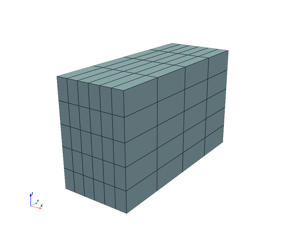
cube = fem.Cube(a=(1, 0, 0), b=(3, 5, 3), n=(7, 5, 6))
cube.plot().show()

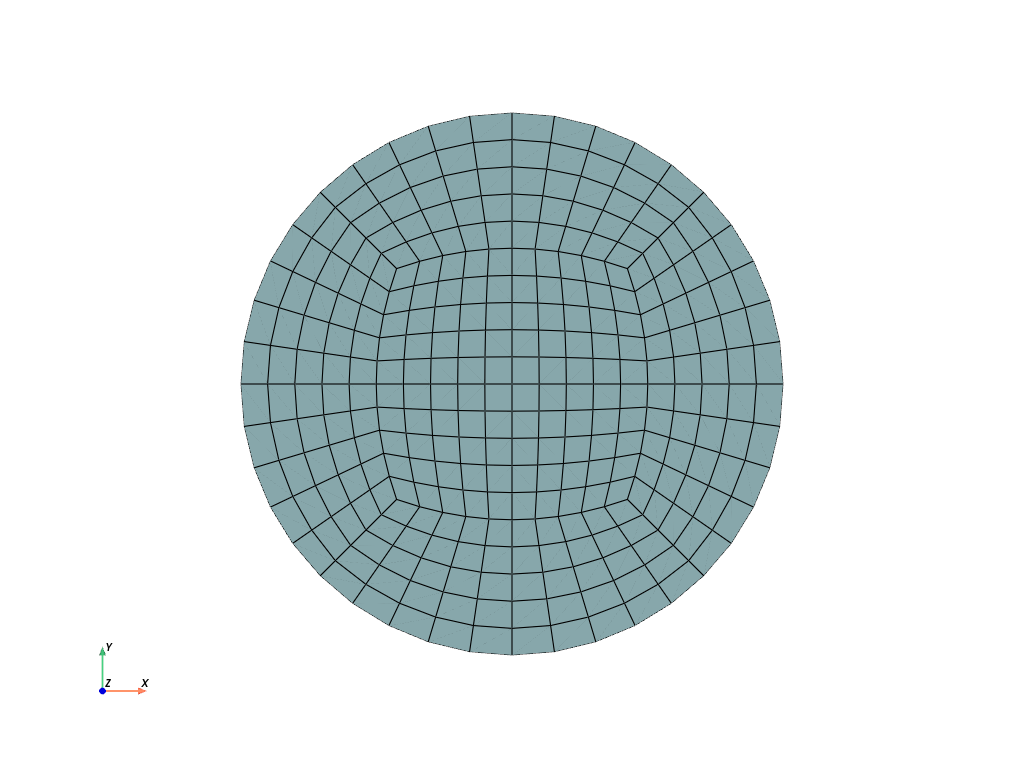
For circles, there is Circle for the creation of a quad-mesh for a circle.
circle = fem.Circle(radius=1.5, centerpoint=[1, 2], n=6, sections=[0, 90, 180, 270])
circle.plot().show()
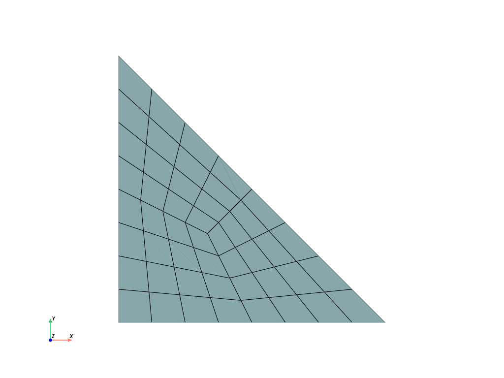
For triangles, there is Triangle for the creation of a quad-mesh for a triangle. For positive cell volumes, the coordinates of a, b and c must be sorted counter-clockwise around the center point.
triangle = fem.mesh.Triangle(a=(0, 0), b=(1, 0), c=(0, 1), n=5)
triangle.plot().show()
Corner Modifications#
For a regular Rectangle or a Cube, corners may be modified by modify_corners(). This is sometimes beneficial for compressive states of deformation.
rectangle = fem.mesh.Rectangle(n=6).modify_corners()
rectangle.plot().show()

Cylinders#
Cylinders are created by a revolution of a rectangle.
r = 25
R = 50
H = 100

rect = fem.Rectangle(a=(-r, 0), b=(-R, H), n=(11, 41))
cylinder = rect.revolve(n=19, phi=-180, axis=1)
cylinder.plot().show()
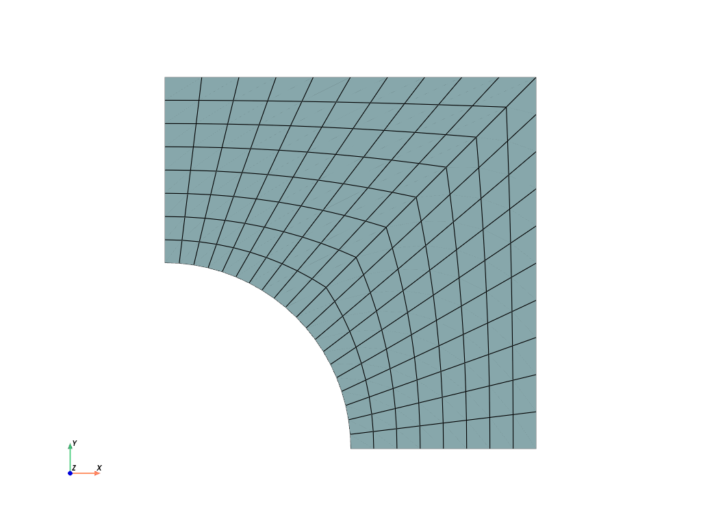
Fill between boundaries#
Meshed boundaries may be used to fill the area or volume in between for line and quad meshes. A plate with a hole is initiated by a line mesh, which is copied two times for the boundaries. The points arrays are updated for the hole and the upper edge. The face is filled by a quad mesh.
n = (11, 9)
phi = np.linspace(1, 0.5, n[0]) * np.pi / 2

line = fem.mesh.Line(n=n[0])
bottom = line.copy(points=0.5 * np.vstack([np.cos(phi), np.sin(phi)]).T)
top = line.copy(
    points=np.vstack([np.linspace(0, 1, n[0]), np.linspace(1, 1, n[0])]).T
)

face = bottom.fill_between(top, n=n[1])
plate_with_hole = fem.mesh.concatenate(
    [face, face.mirror(normal=[-1, 1, 0])]
).merge_duplicate_points()

plate_with_hole.plot().show()
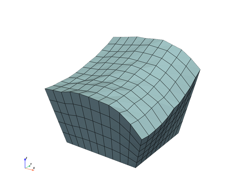
Connect two quad-meshed faces by hexahedrons:
x = np.linspace(0, 1, 11)
y = np.linspace(0, 1, 11)

xg, yg = np.meshgrid(x, y, indexing="ij")
zg = (
    0.5 + 0.3 * xg**2 + 0.5 * yg**2 - 0.7 * yg ** 3 + np.random.rand(11, 11) / 50
)

grid = fem.Grid(x, y)
top = grid.copy(points=np.hstack([grid.points, zg.reshape(-1, 1)]))
bottom = grid.copy(points=np.hstack([grid.points, 0 * zg.reshape(-1, 1)]))

bottom.points += [0.2, 0.1, 0]
bottom.points *= 0.75

mesh = bottom.fill_between(top, n=6)
mesh.plot().show()
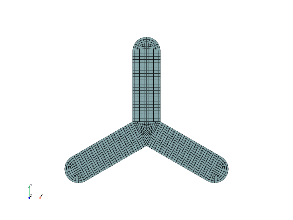
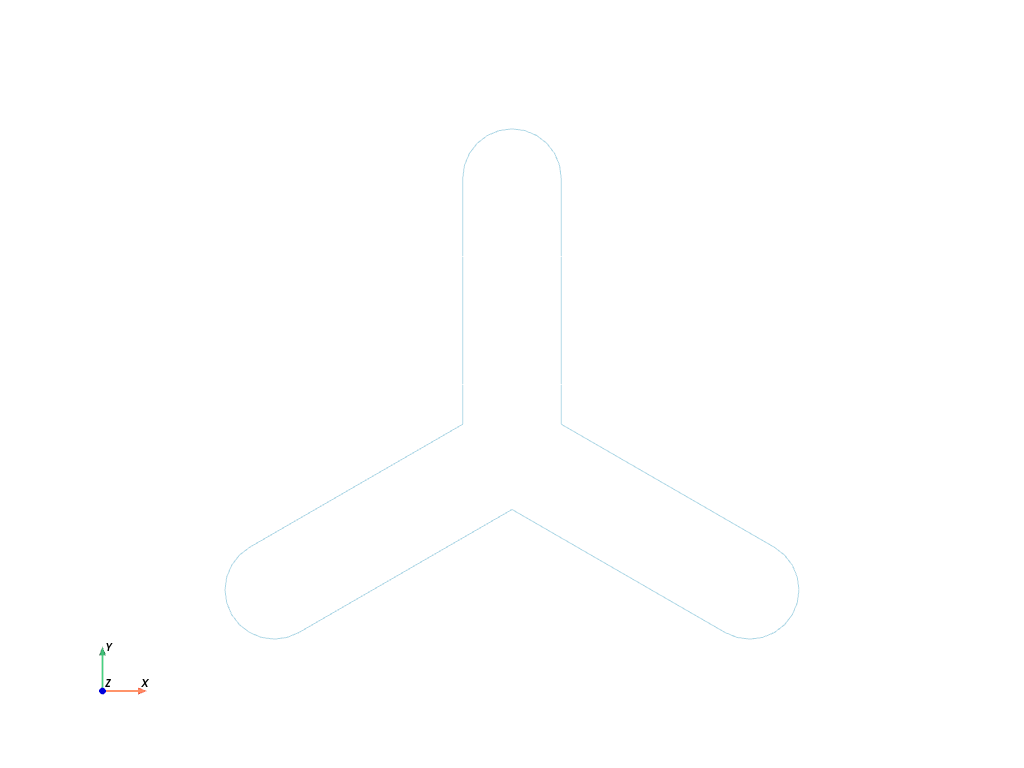
Combinations of elementary shapes#
The elementary shapes are combined to create more complex shapes, e.g. a planar triangular shaped face connected to three arms with rounded ends.
rectangle = fem.Rectangle(a=(-1, 0), b=(1, 5), n=(13, 26))
circle = fem.Circle(radius=1, centerpoint=(0, 5), sections=(0, 90), n=4)
triangle = fem.mesh.Triangle(a=(-1, 0), b=(1, 0), c=(0, -np.sqrt(12) / 2), n=7)
arm = fem.mesh.concatenate([rectangle, circle])

center = triangle.points.mean(axis=0)
arms = [arm.rotate(phi, axis=2, center=center) for phi in [0, 120, 240]]

mesh = fem.mesh.concatenate([triangle, *arms]).merge_duplicate_points(decimals=8)
mesh.plot().show()
For quad- and hexahedron-meshes it is possible to extract the boundaries of the mesh by a boundary region. The boundary-mesh consists of the quad-cells which have their first edge located at the boundary. Hence, these are not the original cells connected to the boundary. The boundary line-mesh is available as a method. In FElupe, boundaries of cell (volumes) are considered as faces and hence, the line-mesh for the edges of a quad-mesh is obtained by a mesh-face method of the boundary region.
boundary = fem.RegionQuadBoundary(mesh)
boundary.mesh.plot().show()
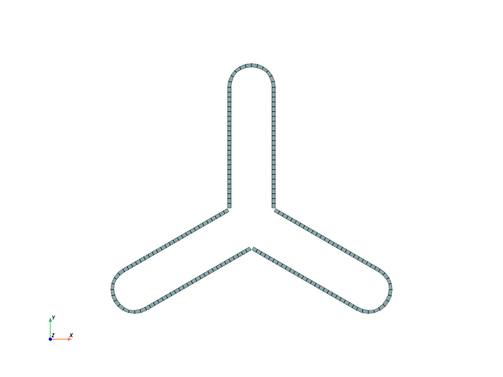
boundary.mesh_faces().plot().show()
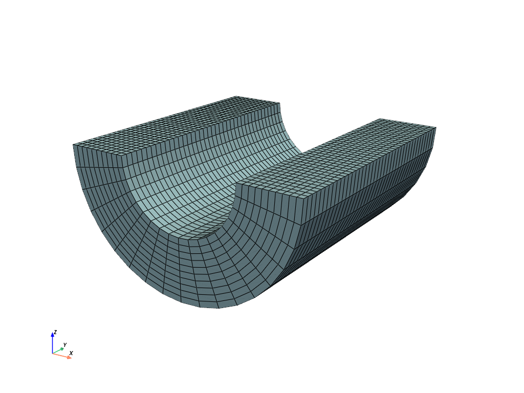
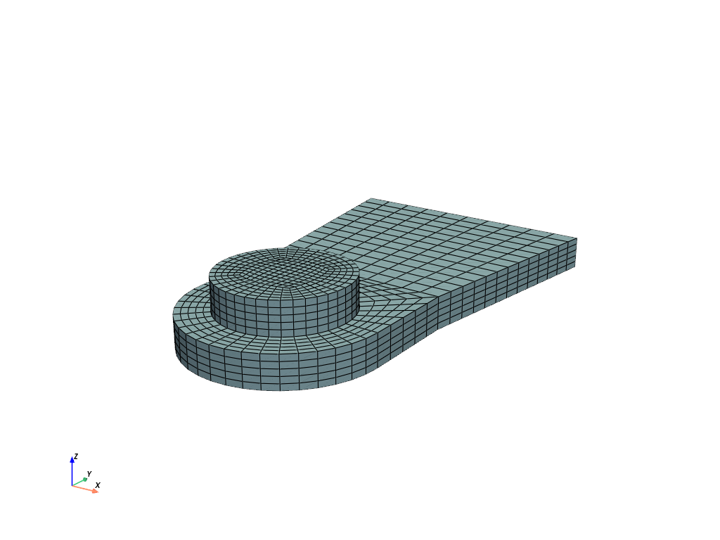
A three-dimensional example demonstrates a combination of two different expansions of a rectangle, fill-betweens of two lines and a circle.
circle = fem.Circle(radius=1, centerpoint=(0, 0), sections=(0, 90, 180, 270), n=6)

phi = np.linspace(1, 0.5, 6) * np.pi / 2

line = fem.mesh.Line(n=6)
curve = line.copy(points=1.0 * np.vstack([np.cos(phi), np.sin(phi)]).T)
top = line.copy(points=np.vstack([np.linspace(0, 1.5, 6), np.linspace(1.5, 1.5, 6)]).T)

transition = curve.fill_between(top, n=6)
transition = fem.mesh.concatenate([transition, transition.mirror(normal=[-1, 1, 0])])

rect = fem.Rectangle(a=(-1.5, 1.5), b=(1.5, 5.0), n=(11, 14))
rect.points[:, 0] *= 1 + (rect.points[:, 1] - 1.5) / 10

face = fem.mesh.concatenate([
    transition,
    transition.mirror(normal=[1, 0, 0]),
    fem.mesh.Line(a=-1.5, b=-1, n=6).revolve(n=21, phi=180, axis=2).flip(),
    rect
])

mesh = fem.mesh.concatenate([
    face.expand(n=6, z=0.5),
    circle.expand(n=11, z=1),
]).merge_duplicate_points(decimals=8)

mesh.plot().show()
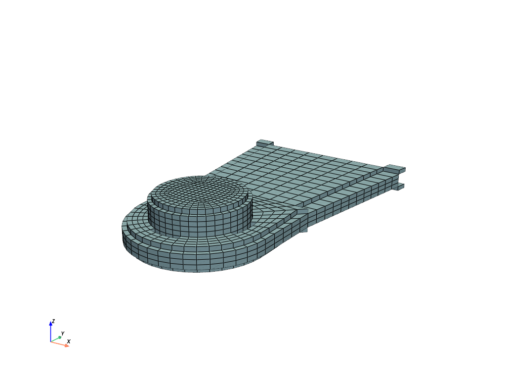
The boundary mesh isn’t visualized correctly in PyVista and in ParaView because there are two duplicated cells at the edges. However, this is not a bug - it’s a feature. Each face on the surface has one attached cell - with the surface face as its first face. Hence, at edges, there are two overlapping cells with different point connectivity.
boundary = fem.RegionHexahedronBoundary(mesh)
boundary.mesh.plot().show()
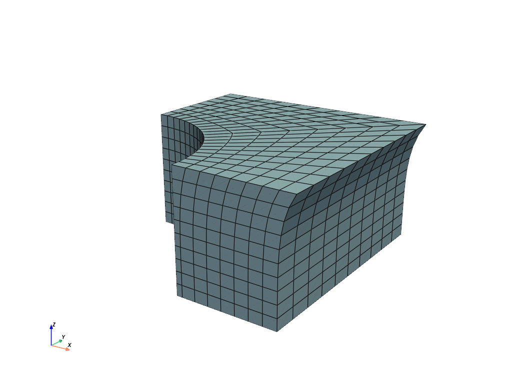
Boundary modification (runouts)#
Indentations (runouts) of the boundary edges or faces are defined by a centerpoint, an axis and their relative amounts (values) per axis. Optionally, the transformation of the point coordinates is restricted to a list of given points.
block = plate_with_hole.expand(z=0.5)
x, y, z = block.points.T

solid = block.add_runouts(
    centerpoint=[0, 0, 0],
    axis=2,
    values=[0.07, 0.02],
    exponent=5,  # shape parameter
    normalize=True,
    mask=np.arange(block.npoints)[np.sqrt(x**2 + y**2) > 0.5]
)
solid.plot().show()
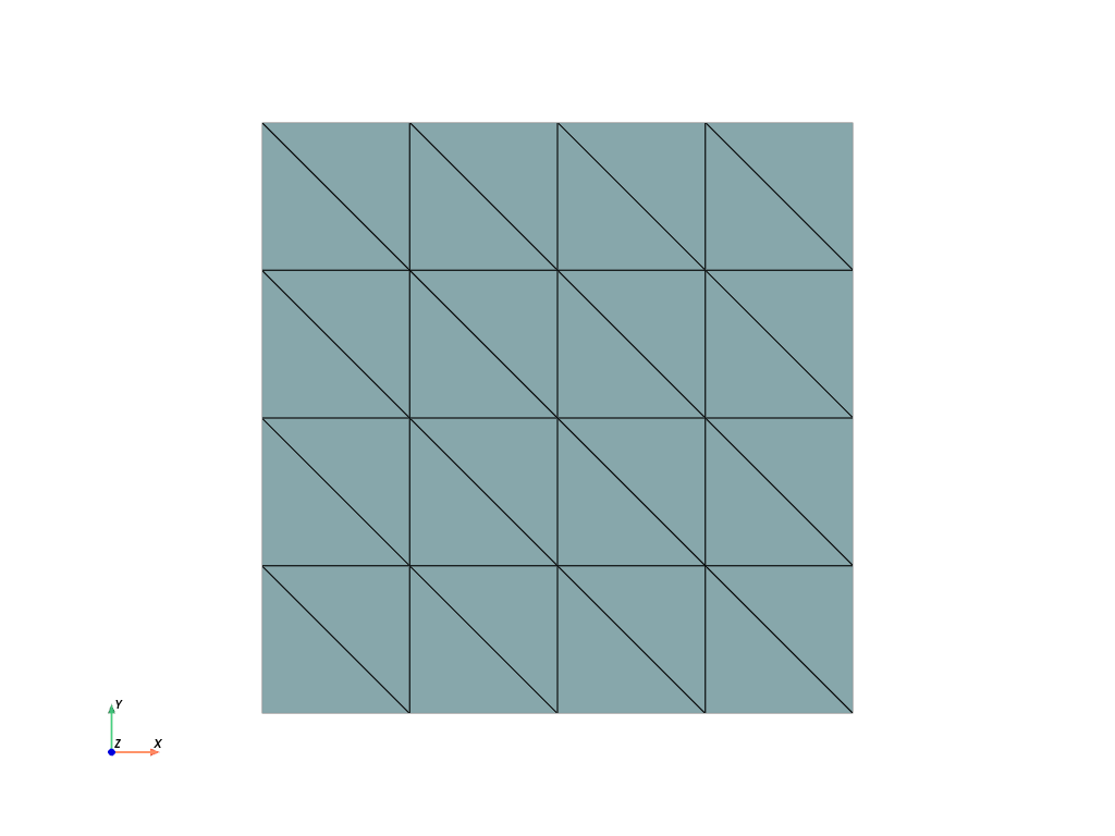
Triangle and Tetrahedron meshes#
Any quad or tetrahedron mesh may be subdivided (triangulated) to meshes out of Triangles or Tetrahedrons by triangulate().
rectangle = fem.Rectangle(n=5).triangulate()
rectangle.plot().show()
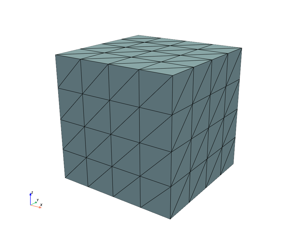
cube = fem.Cube(n=5).triangulate()
cube.plot().show()
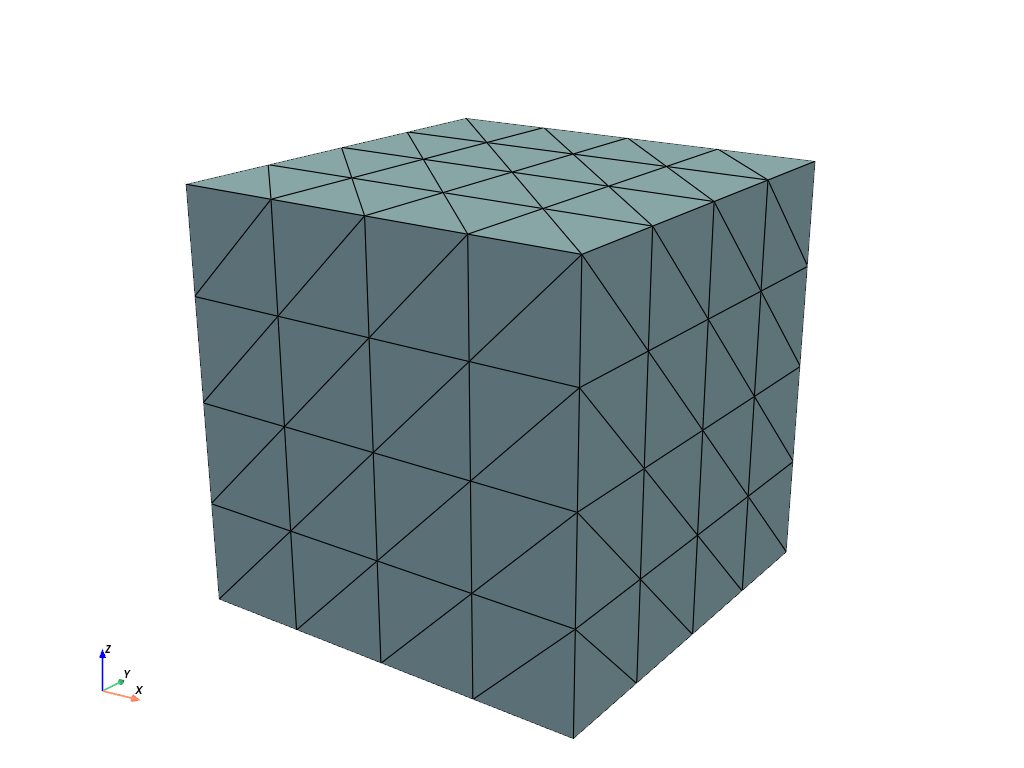
cube = fem.Cube(n=5).triangulate(mode=0)
cube.plot().show()
Meshes with midpoints#
If a mesh with midpoints is required by a region, functions for edge, face and volume midpoint insertions are provided in add_midpoints_edges(), add_midpoints_faces() and add_midpoints_volumes(). A low-order mesh, e.g. a mesh with cell-type quad, can be converted to a quadratic mesh with convert(). By default, only midpoints on edges are inserted. Hence, the resulting cell-type is quad8. If midpoints on faces are also calculated, the resulting cell-type is quad9.
rectangle_quad4 = fem.Rectangle(n=6)
rectangle_quad8 = rectangle_quad4.convert(order=2)
rectangle_quad9 = fem.mesh.convert(rectangle_quad4, order=2, calc_midfaces=True)
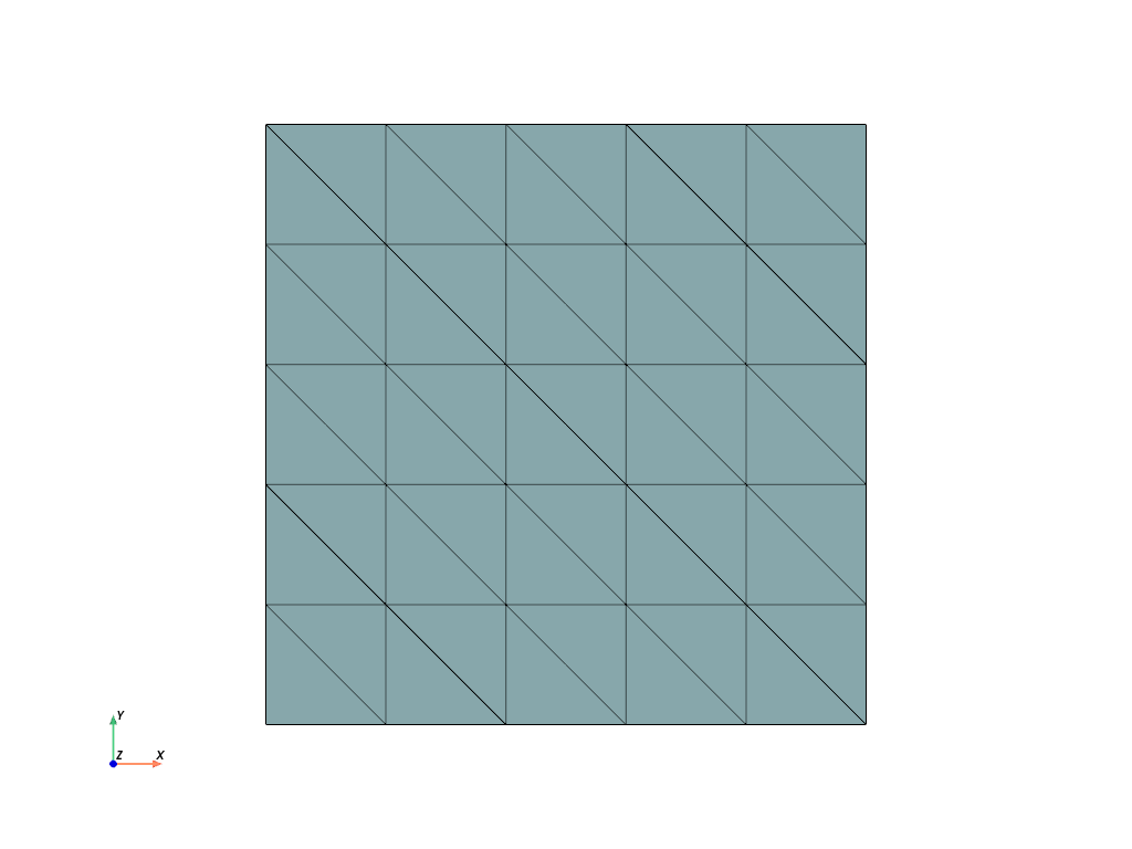
The same also applies on meshes with triangles.
rectangle_triangle3 = fem.Rectangle(n=6).triangulate()
rectangle_triangle6 = rectangle_triangle3.add_midpoints_edges()

rectangle_triangle6.plot(nonlinear_subdivision=2).show()
For views on higher-order meshes use nonlinear_subdivision.