Cantilever beam under gravity

Apply a gravity load on a solid body.

• create a solid body and apply the gravity load

• linear-elastic analysis

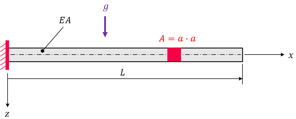
The displacement due to gravity of a cantilever beam with young’s modulus \(E=206000\) MPa, poisson ratio \(\nu=0.3\), length \(L=2000\) mm and cross section area \(A=a \cdot a\) with \(a=100\) mm is to be evaluated within a linear-elastic analysis [1].

First, let’s create a meshed cube out of hexahedron cells with n=(181, 9, 9) points per axis. A numeric region created on the mesh represents the cantilever beam. A three- dimensional vector-valued displacement field is initiated on the region.

import felupe as fem

cube = fem.Cube(a=(0, 0, 0), b=(2000, 100, 100), n=(101, 6, 6))
region = fem.RegionHexahedron(cube, uniform=True)
displacement = fem.Field(region, dim=3)
field = fem.FieldContainer([displacement])

A fixed boundary condition is applied on the left end of the beam.

boundaries = fem.BoundaryDict(fixed=fem.dof.Boundary(displacement, fx=0))
boundaries.plot().show()

Static Scene

Interactive Scene

The material behaviour is defined through a built-in isotropic linear-elastic material formulation.

umat = fem.LinearElastic(E=206000, nu=0.3)
solid = fem.SolidBody(umat=umat, field=field)

The body force is defined by a (constant) gravity field on a solid body.

\[\delta W_{ext} = \int_v \delta \boldsymbol{u} \cdot \rho \boldsymbol{g} ~ dv\]

density = 7850 * 1e-12
gravity = [0, 0, 9810]
force = fem.SolidBodyForce(field, values=gravity, scale=density)

Inside a Newton-Rhapson procedure, the weak form of linear elasticity is assembled into the stiffness matrix and the applied gravity field is assembled into the body force vector.

step = fem.Step(items=[solid, force], boundaries=boundaries)
job = fem.Job(steps=[step]).evaluate()

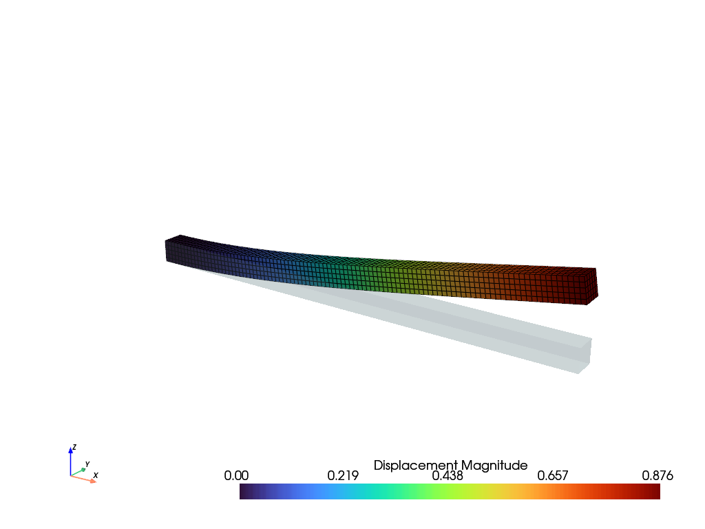
The magnitude of the displacement field are plotted on a 300x scaled deformed configuration.

field.plot("Displacement", component=None, factor=300).show()

Static Scene

Interactive Scene

References

[1]

Glenk C. et al., Consideration of Body Forces within Finite Element Analysis, Strojniški vestnik - Journal of Mechanical Engineering, Faculty of Mechanical Engineering, 2018, .