Non-homogeneous shear

Plane strain hyperelastic non-homogeneous shear loadcase

• define a non-homogeneous shear loadcase

• use a mixed hyperelastic formulation in plane strain

• assign a micro-sphere material formulation

• define a step and a job along with a callback-function

• export and visualize principal stretches

• plot force - displacement curves

This example requires external packages.

pip install matadi

Two rubber blocks of height \(H\) and length \(L\), both glued to a rigid plate on their top and bottom faces, are subjected to a displacement controlled non-homogeneous shear deformation by \(u_{ext}\) in combination with a compressive normal force \(F\).

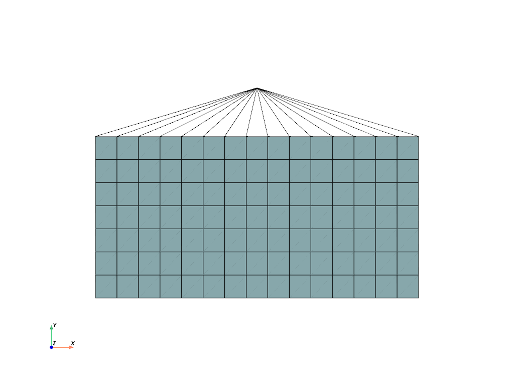
Let’s create the mesh. An additional center-point is created for a multi-point constraint (MPC). By default, FElupe stores points not connected to any cells in Mesh.points_without_cells and adds them to the list of inactive degrees of freedom. Hence, we have to drop our MPC-centerpoint from that list.

import numpy as np

import felupe as fem

H = 10
L = 20
T = 10

n = 11
a = min(L / n, H / n)

mesh = fem.Rectangle((0, 0), (L, H), n=(round(L / a), round(H / a)))
mesh.update(points=np.vstack((mesh.points, [L / 2, 1.3 * H])))
mesh.points_without_cells = np.array([], dtype=bool)

A numeric quad-region created on the mesh in combination with a vector-valued displacement field for plane-strain as well as scalar-valued fields for the hydrostatic pressure and the volume ratio represents the rubber numerically. A shear load case is applied on the displacement field. This involves setting up a y-symmetry plane as well as the absolute value of the prescribed shear movement in direction \(x\) at the MPC-centerpoint.

region = fem.RegionQuad(mesh)
field = fem.FieldsMixed(region, n=3, planestrain=True)

boundaries = {
    "fixed": fem.Boundary(field[0], fy=mesh.y.min()),
    "control": fem.Boundary(field[0], fy=mesh.y.max(), skip=(0, 1)),
}

dof0, dof1 = fem.dof.partition(field, boundaries)

The micro-sphere material formulation is used for the rubber. It is defined as a hyperelastic material in matADi. The material formulation is finally applied on the plane-strain field, resulting in a hyperelastic solid body.

import matadi as mat

umat = mat.MaterialHyperelastic(
    mat.models.miehe_goektepe_lulei,
    mu=0.1475,
    N=3.273,
    p=9.31,
    U=9.94,
    q=0.567,
    bulk=5000.0,
)

rubber = fem.SolidBody(umat=mat.ThreeFieldVariation(umat), field=field)

At the centerpoint of a multi-point constraint (MPC) the external shear movement is prescribed. It also ensures a force-free top plate in direction \(y\).

mpc = fem.MultiPointConstraint(
    field=field,
    points=np.arange(mesh.npoints)[mesh.points[:, 1] == H],
    centerpoint=mesh.npoints - 1,
)

plotter = mesh.plot()
plotter = mpc.plot(plotter=plotter)
plotter.show()

Static Scene

Interactive Scene

The shear movement is applied in substeps, which are each solved with an iterative newton-rhapson procedure. Inside an iteration, the force residual vector and the tangent stiffness matrix are assembled. The fields are updated with the solution of unknowns. The equilibrium is checked as ratio between the norm of residual forces of the active vs. the norm of the residual forces of the inactive degrees of freedom. If convergence is obtained, the iteration loop ends. Both \(y\)-displacement and the reaction force in direction \(x\) of the top plate are saved. This is realized by a callback-function which is called after each successful substep. A step combines all active items along with constant and ramped boundary conditions. Finally, the step is added to a job. A job returns a generator object with the results of all substeps.

UX = fem.math.linsteps([0, 15], 15)
UY = []
FX = []


def callback(stepnumber, substepnumber, substep):
    UY.append(substep.x[0].values[mpc.centerpoint, 1])
    FX.append(substep.fun[2 * mpc.centerpoint] * T)


step = fem.Step(
    items=[rubber, mpc], ramp={boundaries["control"]: UX}, boundaries=boundaries
)
job = fem.Job(steps=[step], callback=callback)
res = job.evaluate()

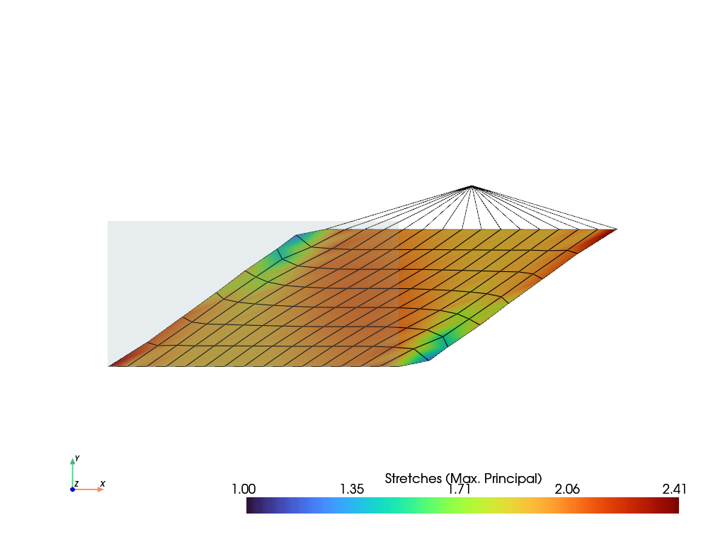
The principal stretches are evaluated for the maximum deformed configuration. This may be done manually, starting from the deformation gradient tensor, or by modifying the FieldContainer.evaluate.strain- method to return the principal stretches. For plotting, these values are projected from quadrature-points to mesh-points.

from felupe.math import dot, eigh, transpose

F = field[0].extract()
C = dot(transpose(F), F)

stretches = np.sqrt(eigh(C)[0])
# stretches = field.evaluate.strain(fun=lambda stretch: stretch, tensor=False)

stretches_at_points = fem.project(stretches, region)
stretches_at_points[-1] = 1  # mpc centerpoint

view = field.view(point_data={"Principal Values of Stretches": stretches_at_points})
plotter = view.plot(
    "Principal Values of Stretches",
    component=0,
)
plotter = mpc.plot(plotter=plotter)
plotter.show()

Static Scene

Interactive Scene

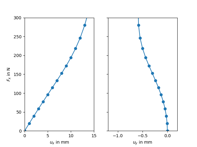
The shear force \(F_x\) vs. the displacements \(u_x\) and \(u_y\), all located at the top plate, are plotted.

import matplotlib.pyplot as plt

fig, ax = plt.subplots(1, 2, sharey=True)

ax[0].plot(UX, FX, "o-")
ax[0].set_xlim(0, 15)
ax[0].set_ylim(0, 300)
ax[0].set_xlabel(r"$u_x$ in mm")
ax[0].set_ylabel(r"$F_x$ in N")

ax[1].plot(UY, FX, "o-")
ax[1].set_xlim(-1.2, 0.2)
ax[1].set_ylim(0, 300)
ax[1].set_xlabel(r"$u_y$ in mm")