Plate with a Hole

Plane stress linear analysis.

• create and mesh a plate with a hole

• define a solid body with a linear-elastic plane stress material

• create an external pressure load

• export and plot stress results

A plate with length \(2L\), height \(2h\) and a hole with radius \(r\) is subjected to a uniaxial tension \(p=-100\) MPa. What is being looked for is the von Mises stress distribution and the concentration of normal stress \(\sigma_{11}\) over the hole.

h = 1
L = 2
r = 0.3

import numpy as np

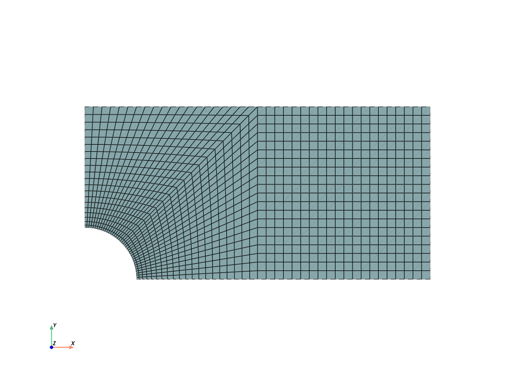
Let’s create a meshed plate with a hole out of quad cells. Only a quarter model of the plate is considered. The mesh generation is carried out by filling the area between the edge of the hole and the top line. Then, this section is duplicated, mirrored and merged with another rectangle.

import felupe as fem

phi = np.linspace(1, 0.5, 21) * np.pi / 2

line = fem.mesh.Line(n=21)
curve = line.copy(points=r * np.vstack([np.cos(phi), np.sin(phi)]).T)
top = line.copy(points=np.vstack([np.linspace(0, h, 21), np.linspace(h, h, 21)]).T)

face = curve.fill_between(top, n=np.linspace(0, 1, 21) ** 1.3 * 2 - 1)
rect = fem.mesh.Rectangle(a=(h, 0), b=(L, h), n=21)
mesh = fem.mesh.concatenate([face, face.mirror(normal=[-1, 1, 0]), rect])
mesh = mesh.sweep(decimals=5)

mesh.plot().show()

Static Scene

Interactive Scene

A numeric quad-region created on the mesh in combination with a vector-valued displacement field represents the plate. The Boundary conditions for the symmetry planes are generated on the displacement field.

region = fem.RegionQuad(mesh)
displacement = fem.Field(region, dim=2)
field = fem.FieldContainer([displacement])

boundaries = fem.dof.symmetry(displacement)

The material behaviour is defined through a built-in isotropic linear-elastic material formulation for plane stress problems. A solid body applies the linear-elastic material formulation on the displacement field.

umat = fem.LinearElasticPlaneStress(E=210000, nu=0.3)
solid = fem.SolidBody(umat, field)

The external uniaxial tension is applied by a pressure load on the right end at \(x=L\). Therefore, a boundary region in combination with a field has to be created at \(x=L\).

region_boundary = fem.RegionQuadBoundary(mesh, mask=mesh.points[:, 0] == L)
field_boundary = fem.FieldContainer([fem.Field(region_boundary, dim=2)])

load = fem.SolidBodyPressure(field_boundary, pressure=-100)

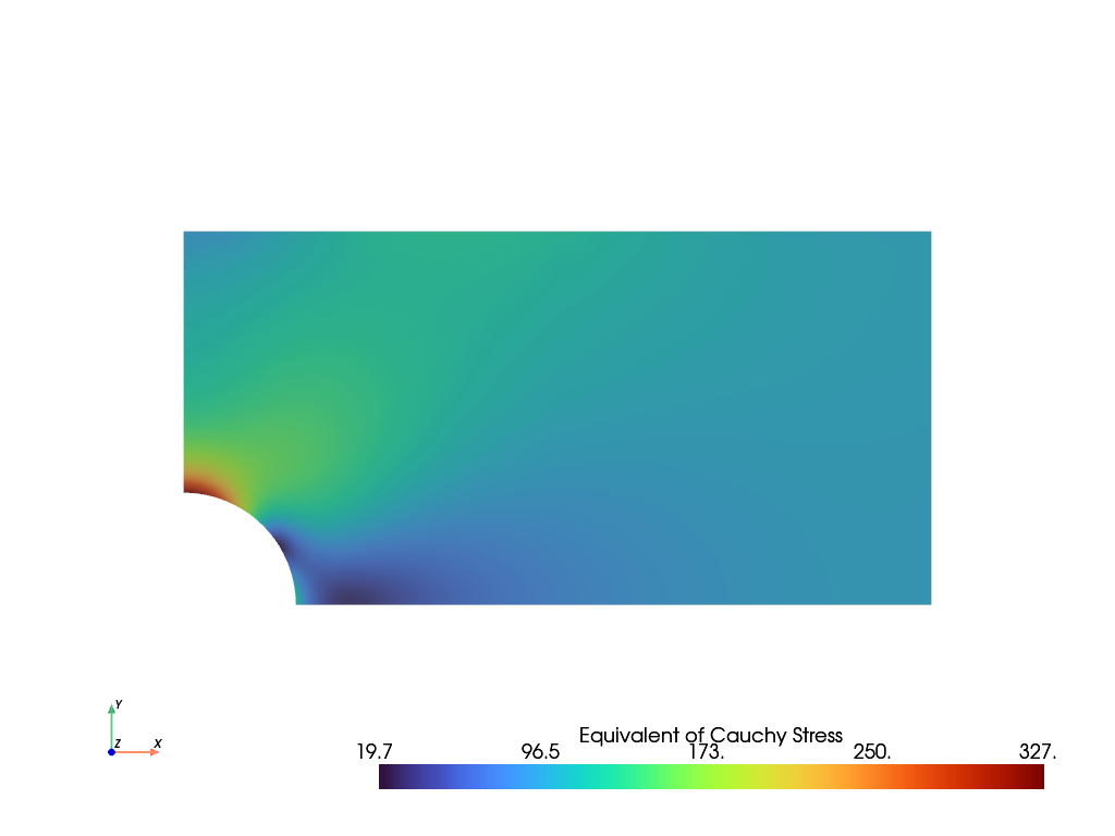
The simulation model is now ready to be solved. The equivalent von Mises Cauchy stress will be plotted. For the two-dimensional case it is calculated by Eq. (1). Stresses, located at quadrature-points of cells, are shifted to and averaged at mesh- points.

(1)\[\sigma_{vM} = \sqrt{\sigma_{11}^2 + \sigma_{22}^2 - \sigma_{11} \ \sigma_{22} + 3 \ \sigma_{12}^2}\]

step = fem.Step(items=[solid, load], boundaries=boundaries)
job = fem.Job(steps=[step]).evaluate()

solid.plot("Equivalent of Cauchy Stress", show_edges=False, project=fem.topoints).show()

Static Scene

Interactive Scene

/home/docs/checkouts/readthedocs.org/user_builds/felupe/envs/latest/lib/python3.11/site-packages/felupe/mechanics/_solidbody.py:345: UserWarning: Cauchy stress tensor can't be evaluated on a 2d-Field.
Falling-back to the Kirchhoff stress tensor.
  warnings.warn(

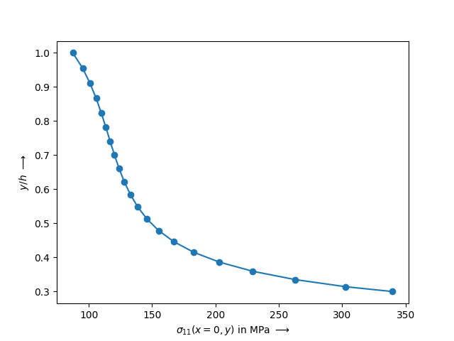
The normal stress distribution \(\sigma_{11}\) over the hole at \(x=0\) is plotted with matplotlib.

import matplotlib.pyplot as plt

plt.plot(
    fem.tools.project(solid.evaluate.cauchy_stress(), region)[:, 0, 0][mesh.x == 0],
    mesh.points[:, 1][mesh.x == 0] / h,
    "o-",
)

plt.xlabel(r"$\sigma_{11}(x=0, y)$ in MPa $\longrightarrow$")
plt.ylabel(r"$y/h$ $\longrightarrow$")

/home/docs/checkouts/readthedocs.org/user_builds/felupe/envs/latest/lib/python3.11/site-packages/felupe/mechanics/_solidbody.py:345: UserWarning: Cauchy stress tensor can't be evaluated on a 2d-Field.
Falling-back to the Kirchhoff stress tensor.
  warnings.warn(