Hyperelastic Spring

A hyperelastic spring with a simplified frictionless contact.

• read a mesh file

• define an isotropic hyperelastic solid body

• setup a simplified frictionless elastic-to-rigid contact interaction

• export and plot the log. strain

This example requires external packages.

pip install pypardiso

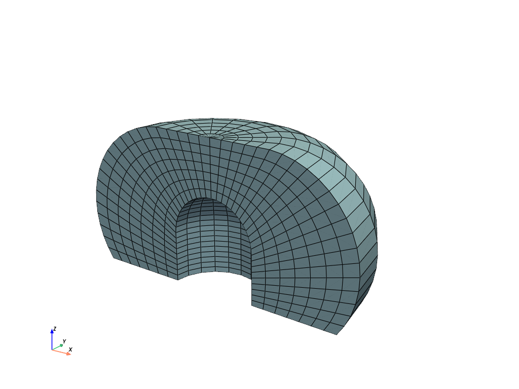
A meshed three-dimensional geometry of a rubber-metal spring is loaded by an external axial and lateral displacement. Simplified elastic-to-rigid contact definitions simulate the end stops caused by steel plates at the bottom and the top in direction \(z\).

import numpy as np
import pypardiso

import felupe as fem

mesh = fem.mesh.read("ex06_rubber-metal-spring_mesh.vtk")[0]
X, Y, Z = mesh.points.T

mesh.plot().show()

Static Scene

Interactive Scene

A numeric hexahedron-region created on the mesh in combination with a vector-valued displacement field represents the volume of the solid. Imported meshes may contain cells with negative volumes. This is fixed as proposed in the warning message. The Boundary conditions for the \(y\)-symmetry plane as well as the fixed faces on the bottom and the top of the solid are generated on the displacement field.

region = fem.RegionHexahedron(mesh)
mesh = mesh.flip(np.any(region.dV < 0, axis=0))

region = fem.RegionHexahedron(mesh)
field = fem.FieldContainer([fem.Field(region, dim=3)])

boundaries = fem.dof.symmetry(field[0], axes=(0, 1, 0))
boundaries["fixed"] = fem.Boundary(field[0], fz=Z.max())
boundaries["move-x"] = fem.Boundary(field[0], fz=Z.min(), skip=(0, 1, 1))
boundaries["move-y"] = fem.Boundary(field[0], fz=Z.min(), skip=(1, 0, 1))
boundaries["move-z"] = fem.Boundary(field[0], fz=Z.min(), skip=(1, 1, 0))

/home/docs/checkouts/readthedocs.org/user_builds/felupe/envs/latest/lib/python3.11/site-packages/felupe/region/_region.py:254: UserWarning: Negative volumes for cells
 [   0    1    2 ... 1467 1468 1469]
Try ``mesh.flip(np.any(region.dV < 0, axis=0))`` and re-create the region.
  warnings.warn(message_negative_volumes)

The material behavior is defined through a built-in hyperelastic isotropic Neo-Hookean material formulation. A solid body applies the material formulation on the displacement field.

umat = fem.NeoHookeCompressible(mu=1, lmbda=5)
solid = fem.SolidBody(umat, field)

The simplified elastic-to-rigid contact is defined by a multi-point constraint-like formulation which is only active in compression. First, the points on the surface of the solid body are determined. Then, the center (control) point is defined by one of the mesh points on the end faces in direction \(z\).

surface = np.unique(fem.RegionHexahedronBoundary(mesh).mesh_faces().cells)
mask = np.isin(np.arange(mesh.npoints), surface)
points = np.where(mask)[0]
bottom = fem.MultiPointContact(
    field,
    points=points,
    centerpoint=np.where(Z == Z.min())[0][0],
    skip=(1, 1, 0),
)
top = fem.MultiPointContact(
    field,
    points=points,
    centerpoint=np.where(Z == Z.max())[0][0],
    skip=(1, 1, 0),
)

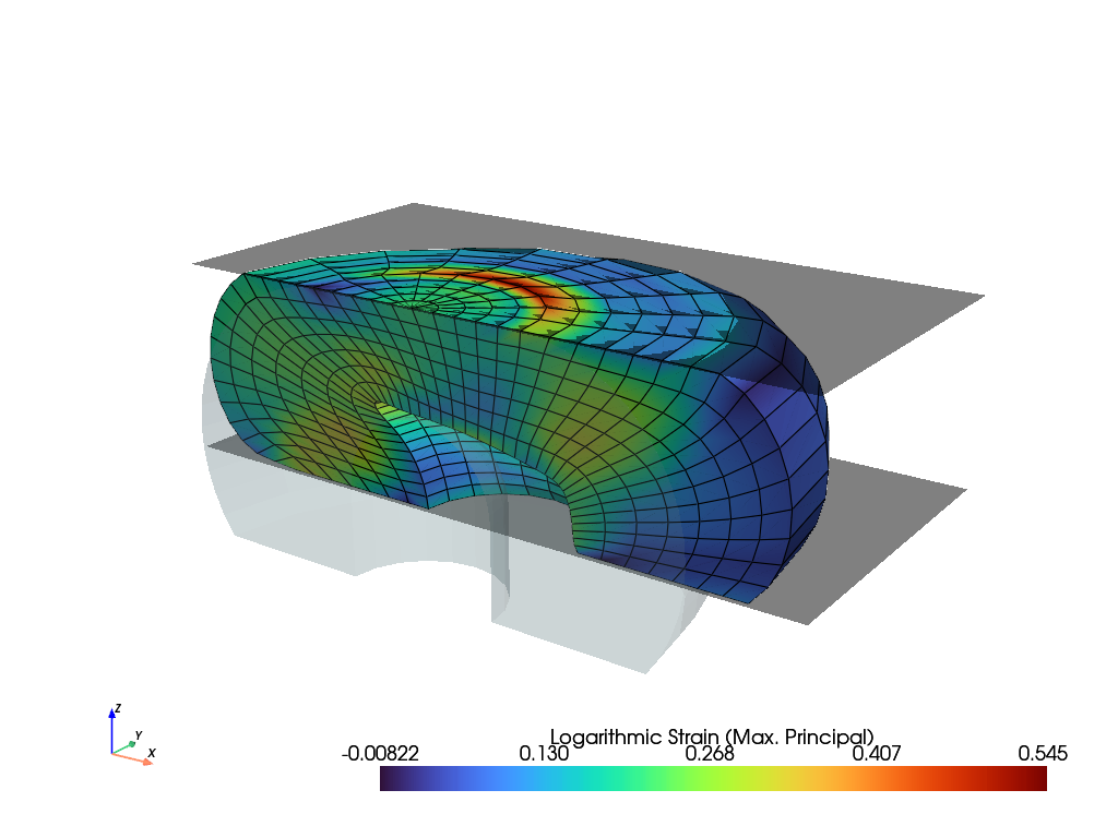
The max. principal value of the logarithmic strain, projected to mesh points, will be added to the result file.

def log_strain(field, substep=None):
    "Project the max. principal log. strain from quadrature- to mesh-points."

    F = field.extract()[0]
    C = fem.math.dot(fem.math.transpose(F), F)
    strain = np.log(fem.math.eigvalsh(C)[-1]) / 2

    return fem.project(strain, region)

The simulation model is now ready to be solved. The results are saved within a XDMF- file, where additional point-data is passed to the point_data argument.

table = fem.math.linsteps([0, 1], num=4)
axial = fem.Step(
    items=[solid, top, bottom],  # , top, bottom
    ramp={boundaries["move-z"]: 40 * table},
    boundaries=boundaries,
)
lateral = fem.Step(
    items=[solid, top, bottom],
    ramp={boundaries["move-x"]: 40 * table},
    boundaries=boundaries,
)
job = fem.CharacteristicCurve(steps=[axial, lateral], boundary=boundaries["move-z"])
job.evaluate(
    filename="result.xdmf",
    solver=pypardiso.spsolve,
    point_data={"Logarithmic Strain (Max. Principal)": log_strain},
    tol=1e-1,
)
view = field.view(
    point_data={"Logarithmic Strain (Max. Principal)": log_strain(field)},
)
plotter = view.plot("Logarithmic Strain (Max. Principal)")
plotter = top.plot(plotter=plotter, offset=1e-1)
plotter = bottom.plot(plotter=plotter, offset=-1e-1)
plotter.show()

Static Scene

Interactive Scene

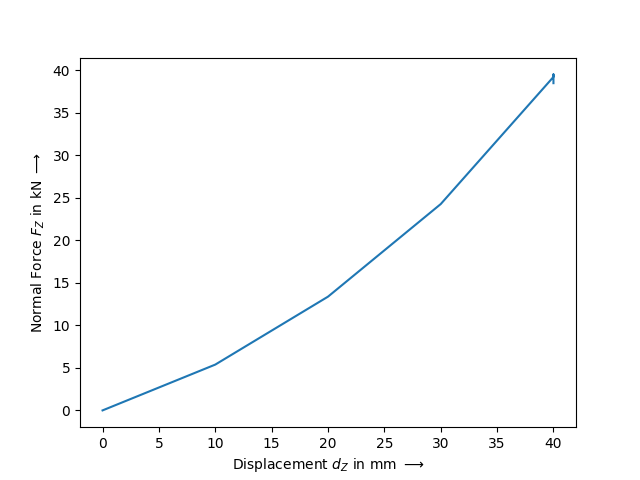
The axial-compressive and lateral-shear force-displacement curves are obtained from the characteristic-curve job. The force is multiplied by two due to the fact that only one half of the geometry is simulated.

fig, ax = job.plot(
    xlabel="Displacement $d_Z$ in mm $\longrightarrow$",
    ylabel="Normal Force $F_Z$ in kN $\longrightarrow$",
    xaxis=2,
    yaxis=2,
    yscale=2 / 1000,
)

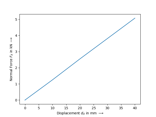
The shear lateral force-displacement curve is again obtained from the characteristic- curve job.

fig, ax = job.plot(
    xlabel="Displacement $d_X$ in mm $\longrightarrow$",
    ylabel="Normal Force $F_X$ in kN $\longrightarrow$",
    xaxis=0,
    yaxis=0,
    yscale=2 / 1000,
)