Plasticity with Isotropic Hardening

Small-strain Plasticity

• linear-elastic plastic material formulation with isotropic hardening

• define a body force vector

• extract state variables

The normal plastic strain due to a body force applied on a solid with a linear-elastic plastic material formulation with isotropic hardening with young’s modulus \(E=210000\), poisson ratio \(\nu=0.3\), isotropic hardening modulus \(K=1000\), yield stress \(\sigma_y=355\), length \(L=3\) and cross section area \(A=1\) is to be evaluated.

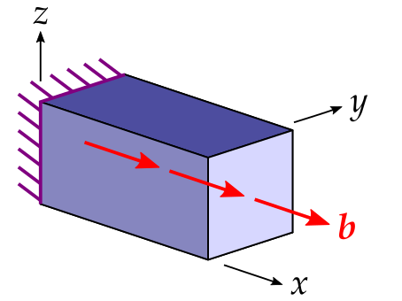
First, let’s create a meshed cube out of hexahedron cells with n=(16, 6, 6) points per axis. A three-dimensional vector-valued displacement field is initiated on the numeric region.

import numpy as np

import felupe as fem

mesh = fem.Cube(b=(3, 1, 1), n=(16, 6, 6))
region = fem.RegionHexahedron(mesh)
displacement = fem.Field(region, dim=3)
field = fem.FieldContainer([displacement])

A fixed boundary condition is applied at \(x=0\).

boundaries = {"fixed": fem.dof.Boundary(displacement, fx=0)}

The material behaviour is defined through a built-in isotropic linear-elastic plastic material formulation with isotropic hardening.

umat = fem.LinearElasticPlasticIsotropicHardening(E=2.1e5, nu=0.3, sy=355, K=1e3)
solid = fem.SolidBody(umat, field)

The body force is created on the field of the solid body.

\[\delta W_{ext} = \int_v \delta \boldsymbol{u} \cdot \boldsymbol{b} ~ dv\]

bodyforce = fem.SolidBodyGravity(field)
b = fem.math.linsteps([0, 200], num=10, axis=0, axes=3)

Inside a Newton-Rhapson procedure, the vectors and matrices are assembled for the given items and the boundary conditions are incorporated into the equilibrium equations.

step = fem.Step(items=[solid, bodyforce], ramp={bodyforce: b}, boundaries=boundaries)
job = fem.Job(steps=[step]).evaluate()

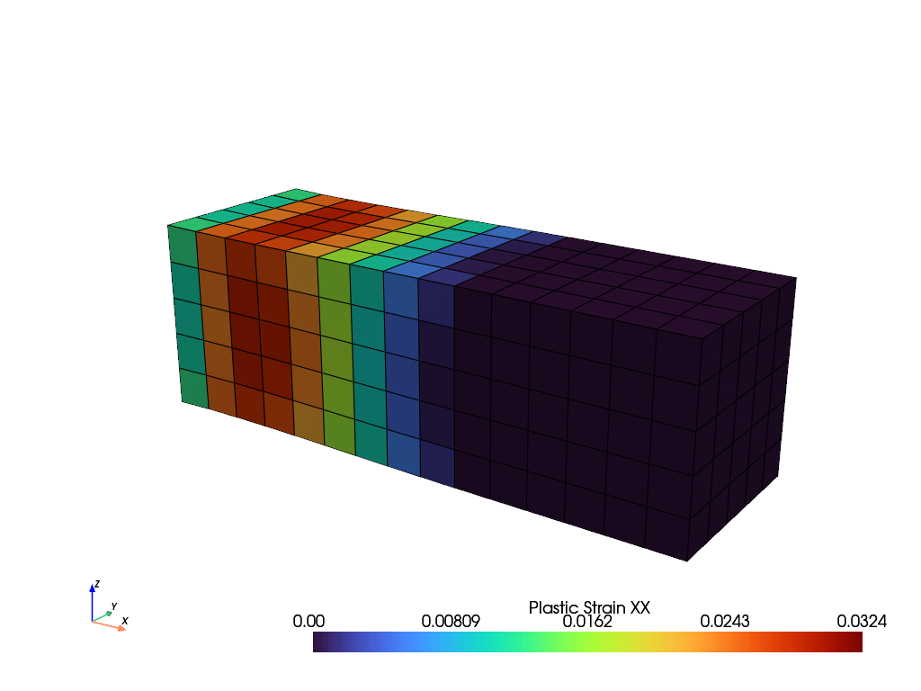
A view on the field-container shows the deformed mesh and the normal plastic strain in direction \(x\) due to the applied body force. The vector of all state variables, stored as a result in the solid body object, are splitted into separate variables. The plastic strain is stored as the second state variable. The mean-per-cell value of the plastic strain in direction \(x\) is exported to the view.

def plot(solid, field):
    "Visualize the final Normal Plastic Strain in direction X."

    plastic_strain = np.split(solid.results.statevars, umat.statevars_offsets)[1]
    view = fem.View(field, cell_data={"Plastic Strain": plastic_strain.mean(-2).T})
    return view.plot("Plastic Strain", component=0, show_undeformed=False)


plot(solid, field).show()

Static Scene

Interactive Scene