Numeric Continuation#

With the help of contique (install with pip install contique) it is possible to apply a numerical parameter continuation algorithm on any system of equilibrium equations. This example demonstrates the usage of FElupe in conjunction with contique. An unstable isotropic hyperelastic material formulation is applied on a single hexahedron. The model will be visualized and the resulting force - displacement curve will be plotted.

import contique
import matplotlib.pyplot as plt
import meshio
import numpy as np

import felupe as fem
import felupe.constitution.tensortrax as mat

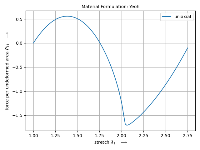
First, setup a problem as usual (mesh, region, field, boundaries and umat). The unstable material behavior is plotted for uniaxial incompressible tension.

# setup a numeric region on a cube
mesh = fem.Cube(n=2)
region = fem.RegionHexahedron(mesh)
field = fem.FieldContainer([fem.Field(region, dim=3)])

# introduce symmetry planes at x=y=z=0
bounds = fem.dof.symmetry(field[0], axes=(True, True, True))

# partition degrees of freedom
dof0, dof1 = fem.dof.partition(field, bounds)

# constitutive isotropic hyperelastic material formulation
yeoh = mat.Hyperelastic(mat.models.hyperelastic.yeoh, C10=0.5, C20=-0.25, C30=0.025)
ax = yeoh.plot(incompressible=True, ux=np.linspace(1, 2.76), bx=None, ps=None)
body = fem.SolidBodyNearlyIncompressible(yeoh, field, bulk=5000)

Hyperelastic (Yeoh), C10=0.5, C20=-0.25, C30=0.025

An external normal force is applied at \(x=1\) on a quarter model of a cube with symmetry planes at \(x=y=z=0\). Therefore, we have to define an external load vector which will be scaled with the load-proportionality factor \(\lambda\) during numeric continuation.

# external force vector at x=1
right = region.mesh.points[:, 0] == 1
v = region.mesh.cells_per_point[right]
values_load = np.vstack([v, np.zeros_like(v), np.zeros_like(v)]).T

load = fem.PointLoad(field, right, values_load)

The next step involves the problem definition for contique. For details have a look at contique’s README.

def fun(x, lpf, *args):
    "The system vector of equilibrium equations."

    # re-create field-values from active degrees of freedom
    body.field[0].values.fill(0)
    body.field[0].values.ravel()[dof1] += x
    load.update(values_load * lpf)

    return fem.tools.fun(items=[body, load], x=body.field)[dof1]


def dfundx(x, lpf, *args):
    """The jacobian of the system vector of equilibrium equations w.r.t. the
    primary unknowns."""

    body.field[0].values.fill(0)
    body.field[0].values.ravel()[dof1] += x
    load.update(values_load * lpf)

    r = fem.tools.fun(items=[body, load], x=body.field)
    K = fem.tools.jac(items=[body, load], x=body.field)

    return fem.solve.partition(body.field, K, dof1, dof0, r)[2]


def dfundl(x, lpf, *args):
    """The jacobian of the system vector of equilibrium equations w.r.t. the
    load proportionality factor."""

    load.update(values_load)

    return fem.tools.fun(items=[load], x=body.field)[dof1]

Next we have to init the problem and specify the initial values of unknowns (the undeformed configuration). After each completed step of the numeric continuation the XDMF-file will be updated.

# write xdmf file during numeric continuation
with meshio.xdmf.TimeSeriesWriter("result.xdmf") as writer:
    writer.write_points_cells(mesh.points, [(mesh.cell_type, mesh.cells)])

    def step_to_xdmf(step, res):
        writer.write_data(step, point_data={"u": field[0].values})

    # run contique (w/ rebalanced steps, 5% overshoot and a callback function)
    Res = contique.solve(
        fun=fun,
        jac=[dfundx, dfundl],
        x0=field[0][dof1],
        lpf0=0,
        dxmax=0.06,
        dlpfmax=0.02,
        maxsteps=35,
        rebalance=True,
        overshoot=1.05,
        callback=step_to_xdmf,
        tol=1e-2,
    )

    X = np.array([res.x for res in Res])

# check the final lpf value
assert np.isclose(X[-1, 1], -0.3982995)

|Step,C.| Control Component | Norm (Iter.#) | Message     |
|-------|-------------------|---------------|-------------|
|   1,1 |    12+  =>    12+ | 1.1e-03 ( 2#) |             |
|   2,1 |    12+  =>    12+ | 1.3e-03 ( 2#) |             |
|   3,1 |    12+  =>    12+ | 1.5e-03 ( 2#) |             |
|   4,1 |    12+  =>    12+ | 7.8e-03 ( 2#) |             |
|   5,1 |    12+  =>    12+ | 1.5e-04 ( 4#) |             |
|   6,1 |    12+  =>     9- | 5.4e+02 ( 8#) |Failed       |
|   7,1 |    12+  =>    12+ | 1.1e-01 ( 8#) |Failed       |
|   8,1 |    12+  =>     9+ | 3.2e-03 ( 2#) | => re-Cycle |
|     2 |     9+  =>     9+ | 1.4e-03 ( 2#) |             |
|   9,1 |     9+  =>     0+ | 1.3e-03 ( 2#) |tol.Overshoot|
|  10,1 |     0+  =>     2+ | 1.1e-03 ( 2#) |tol.Overshoot|
|  11,1 |     2+  =>     9+ | 3.6e-03 ( 2#) |tol.Overshoot|
|  12,1 |     9+  =>     0+ | 1.8e-08 ( 3#) |tol.Overshoot|
|  13,1 |     0+  =>     5+ | 1.1e-07 ( 3#) |tol.Overshoot|
|  14,1 |     5+  =>    12- | 6.1e-07 ( 3#) | => re-Cycle |
|     2 |    12-  =>    12- | 3.4e-03 ( 4#) |             |
|  15,1 |    12-  =>    12- | 1.5e-04 ( 4#) |             |
|  16,1 |    12-  =>    12- | 8.9e-06 ( 4#) |             |
|  17,1 |    12-  =>    12- | 4.0e-06 ( 4#) |             |
|  18,1 |    12-  =>    12- | 5.4e-03 ( 3#) |             |
|  19,1 |    12-  =>    12- | 8.5e-03 ( 4#) |             |
|  20,1 |    12-  =>    12- | 1.0e+02 ( 8#) |Failed       |
|  21,1 |    12-  =>     0- | 8.5e+07 ( 8#) |Failed       |
|  22,1 |    12-  =>     9+ | 6.3e-01 ( 8#) |Failed       |
|  23,1 |    12-  =>    12- | 8.3e-03 ( 3#) |             |
|  24,1 |    12-  =>    12- | 1.4e+01 ( 8#) |Failed       |
|  25,1 |    12-  =>     0+ | 2.6e-03 ( 3#) | => re-Cycle |
|     2 |     0+  =>     5+ | 6.0e-05 ( 2#) |tol.Overshoot|
|  26,1 |     5+  =>     0+ | 5.7e-05 ( 2#) |tol.Overshoot|
|  27,1 |     0+  =>     2+ | 5.5e-05 ( 2#) |tol.Overshoot|
|  28,1 |     2+  =>     9+ | 1.9e-04 ( 2#) |tol.Overshoot|
|  29,1 |     9+  =>     2+ | 6.3e-04 ( 2#) |tol.Overshoot|
|  30,1 |     2+  =>    12+ | 2.1e-03 ( 2#) | => re-Cycle |
|     2 |    12+  =>    12+ | 1.9e-05 ( 4#) |             |
|  31,1 |    12+  =>    12+ | 6.6e-04 ( 3#) |             |
|  32,1 |    12+  =>    12+ | 1.8e-04 ( 3#) |             |
|  33,1 |    12+  =>    12+ | 8.3e-05 ( 3#) |             |
|  34,1 |    12+  =>    12+ | 5.4e-05 ( 3#) |             |
|  35,1 |    12+  =>    12+ | 4.2e-05 ( 3#) |             |

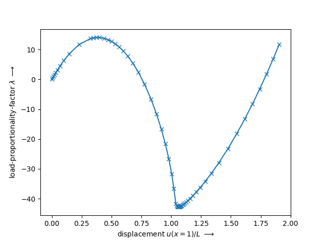
Finally, the force-displacement curve is plotted. It can be seen that the resulting (unstable) force-controlled equilibrium path is equal to the displacement-controlled load case.

plt.figure()
plt.plot(X[:, 0], X[:, -1], "x-")
plt.xlabel(r"displacement $u(x=1)/L$ $\longrightarrow$")
plt.ylabel(r"load-proportionality-factor $\lambda$ $\longrightarrow$")

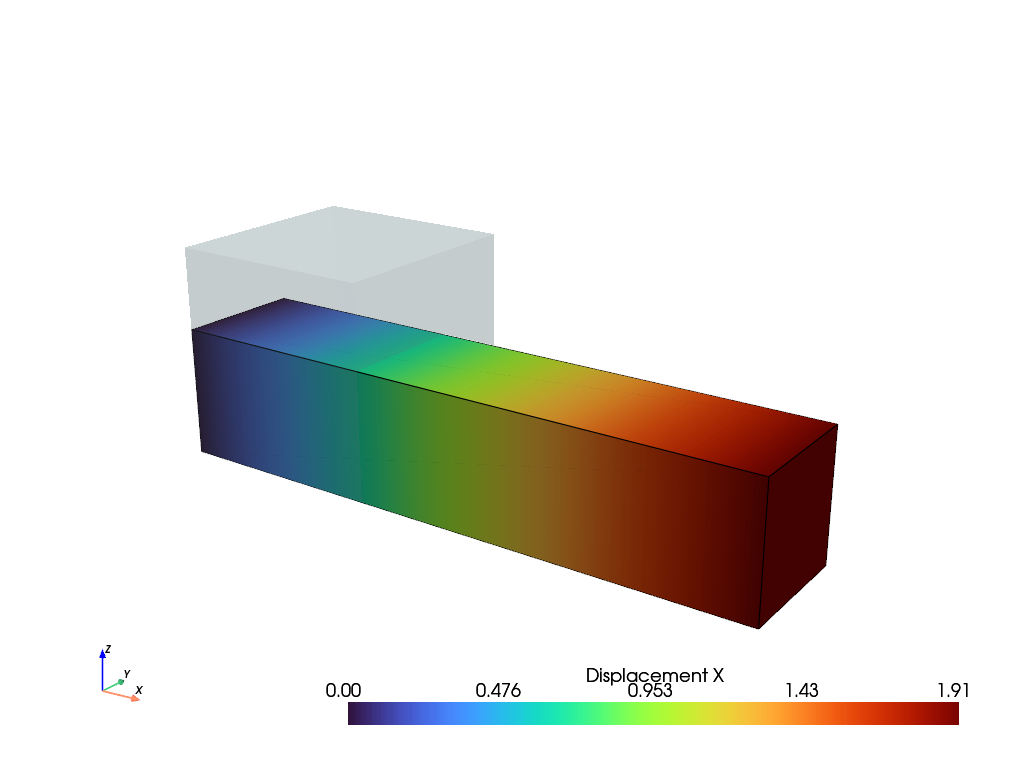
field.plot("Displacement", component=0).show()