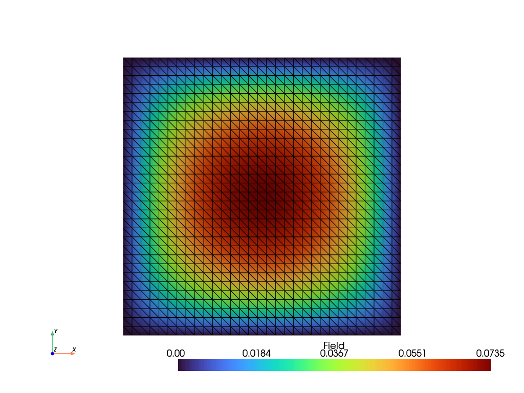
Poisson Equation

The Poisson equation

\[\text{div}(\boldsymbol{\nabla} v) + f = 0 \quad \text{in} \quad \Omega\]

with fixed boundaries on the bottom, top, left and right end-edges

\[v = 0 \quad \text{on} \quad \Gamma_v\]

and a unit load

\[f = 1 \quad \text{in} \quad \Omega\]

is solved on a unit rectangle with triangles.

The Poisson equation is transformed into integral form representation by the divergence (Gauss’s) theorem.

\[\int_\Omega \boldsymbol{\nabla} v \cdot \boldsymbol{\nabla} u \ d\Omega = \int_\Omega f \cdot v \ d\Omega\]

For the newtonrhapson() to converge, the linear form of the Poisson equation is also required.

import felupe as fem
from felupe.math import ddot, grad

mesh = fem.Rectangle(n=2**5).triangulate()
region = fem.RegionTriangle(mesh)
scalar = fem.Field(region)
field = fem.FieldContainer([scalar])


@fem.Form(v=field, u=field)
def a():
    "Container for a bilinear form."
    return [lambda v, u, **kwargs: ddot(grad(v), grad(u))]


@fem.Form(v=field)
def L():
    "Container for a linear form."
    return [lambda v, **kwargs: ddot(grad(v), grad(scalar)) - kwargs["scale"] * v]


poisson = fem.FormItem(bilinearform=a, linearform=L, kwargs={"scale": 1.0})

boundaries = {
    "bottom-or-left": fem.Boundary(field[0], fx=0, fy=0, mode="or"),
    "top-or-right": fem.Boundary(field[0], fx=1, fy=1, mode="or"),
}

step = fem.Step([poisson], boundaries=boundaries)
job = fem.Job([step]).evaluate()

view = mesh.view(point_data={"Field": scalar.values})
view.plot("Field", show_undeformed=False).show()

Static Scene

Interactive Scene