Engine Mount

A rubberlike-metal component used as an engine-mount.

• read and combine mesh files

• define an isotropic hyperelastic solid body

• create consecutive steps and add them to a job

• export and plot characteristic curves

An engine-mount is loaded by a combined vertical and horizontal displacement. What is being looked for are the characteristic force-displacement curves in vertical and horizontal directions as well as the logarithmic strain distribution inside the rubber. The air inside the structure is meshed as a hyperelastic solid with no volumetric part of the strain energy function for a simplified treatment of the rubber contact. The metal parts are simplified as rigid bodies. Three mesh files are provided for this example:

• a mesh for the metal parts,

• a mesh for the rubber blocks as well as

• a mesh for the air inside the engine mount.

import numpy as np

import felupe as fem

metal = fem.mesh.read("ex07_engine-mount_mesh-metal.vtk", dim=2)[0]
rubber = fem.mesh.read("ex07_engine-mount_mesh-rubber.vtk", dim=2)[0]
air = fem.mesh.read("ex07_engine-mount_mesh-air.vtk", dim=2)[0]

# sub-meshes with shared points-array and a global mesh
meshes = fem.MeshContainer([metal, rubber, air], merge=True)
mesh = fem.mesh.concatenate(meshes).sweep()
meshes.plot(colors=["grey", "black", "white"]).show()

Static Scene

Interactive Scene

A global region as well as sub-regions for all materials are generated. The same applies to the fields.

region = fem.RegionQuad(mesh)
regions = [fem.RegionQuad(m) for m in meshes]

field = fem.FieldsMixed(region, n=1, planestrain=True)
fields = [fem.FieldsMixed(r, n=1, planestrain=True) for r in regions]
[f.link(field) for f in fields]

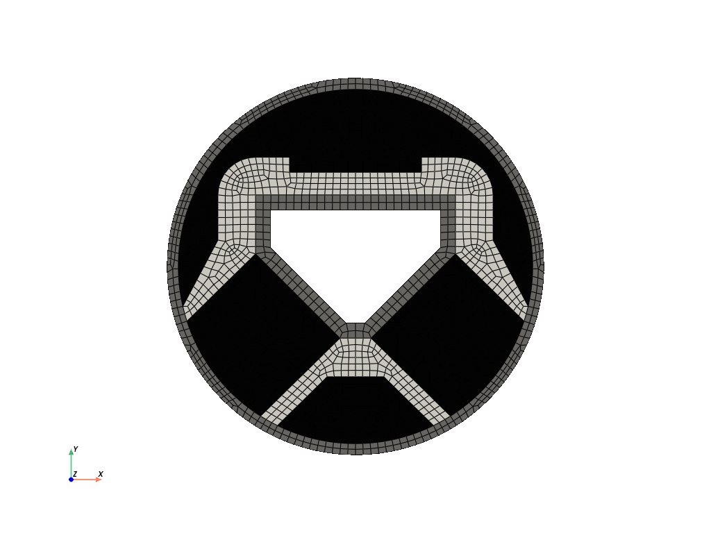
The boundary conditions are created on the global displacement field. First, a mask for all points related to the metal parts is created. Then, this mask is splitted into the inner and the outer metal part.

x, y = mesh.points.T
radius = np.sqrt(x**2 + y**2)

only_cells_metal = np.isin(np.arange(mesh.npoints), np.unique(meshes[0].cells))
inner = np.logical_and(only_cells_metal, radius <= 45)
outer = np.logical_and(only_cells_metal, radius > 45)

boundaries = dict(
    fixed=fem.Boundary(field[0], mask=outer),
    u_x=fem.Boundary(field[0], mask=inner, skip=(0, 1)),
    u_y=fem.Boundary(field[0], mask=inner, skip=(1, 0)),
)

The material behaviour of the rubberlike solid is defined through a built-in hyperelastic isotropic compressible Neo-Hookean material formulation. A solid body applies the material formulation on the displacement field. The air is also simulated by a Neo-Hookean material formulation but with no volumetric contribution and hence, no special mixed-field treatment is necessary here. A crucial parameter is the shear modulus which is used for the simulation of the air. The air is meshed and simulated to capture the contacts of the rubber blocks inside the engine mount during the deformation. Hence, its overall stiffness contribution must be as low as possible. Here, 1 / 25 of the shear modulus of the rubber is used. The bulk modulus of the rubber is lowered to provide a more realistic deformation for the three-dimensional component simulated by a plane- strain analysis.

shear_modulus = 1
rubber = fem.SolidBodyNearlyIncompressible(
    umat=fem.NeoHooke(mu=shear_modulus), field=fields[1], bulk=100
)
air = fem.SolidBody(umat=fem.NeoHooke(mu=shear_modulus / 25), field=fields[2])

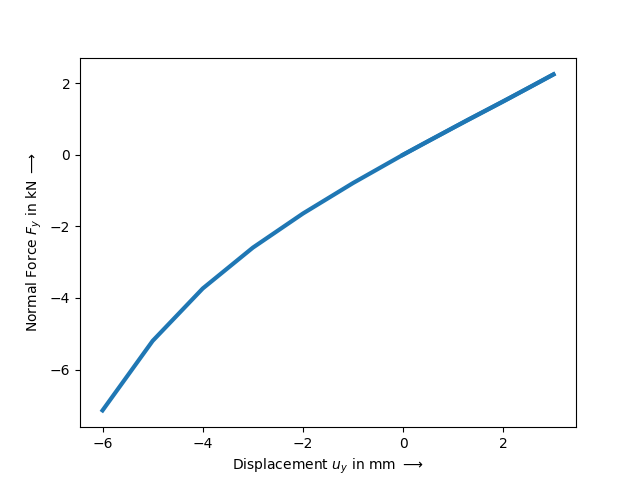
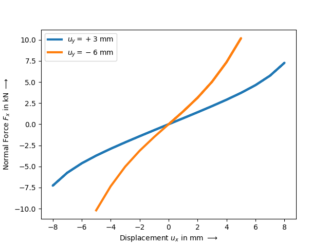
After defining the consecutive load steps, the simulation model is ready to be solved. As we are not interested in the strains of the simulated air, a trimmed mesh is specified during the evaluation of the characteristic-curve job. The lateral force- displacement curves are plotted for the two different levels of vertical displacement.

thickness = 100
vertical = fem.Step(
    items=[rubber, air],
    ramp={boundaries["u_y"]: fem.math.linsteps([0, 3], num=3)},
    boundaries=boundaries,
)
job = fem.CharacteristicCurve(steps=[vertical], boundary=boundaries["u_y"]).evaluate(
    x0=field, tol=1e-1
)
figv, axv = job.plot(
    xlabel="Displacement $u_y$ in mm $\longrightarrow$",
    ylabel="Normal Force $F_y$ in kN $\longrightarrow$",
    xaxis=1,
    yaxis=1,
    yscale=1 / 1000 * thickness,
    ls="-",
    lw=3,
)

horizontal = fem.Step(
    items=[rubber, air],
    ramp={boundaries["u_x"]: 8 * fem.math.linsteps([0, 1, 0, -1, 0], num=8)},
    boundaries=boundaries,
)
job = fem.CharacteristicCurve(steps=[horizontal], boundary=boundaries["u_y"]).evaluate(
    x0=field, tol=1e-1
)
figh, axh = job.plot(
    xlabel="Displacement $u_x$ in mm $\longrightarrow$",
    ylabel="Normal Force $F_x$ in kN $\longrightarrow$",
    yscale=1 / 1000 * thickness,
    lw=3,
    color="C0",
    label=r"$u_y=+3$ mm",
)

vertical = fem.Step(
    items=[rubber, air],
    ramp={boundaries["u_y"]: fem.math.linsteps([3, 0, -6], num=[7, 6])},
    boundaries=boundaries,
)
job = fem.CharacteristicCurve(steps=[vertical], boundary=boundaries["u_y"]).evaluate(
    x0=field, tol=1e-1
)
figv, axv = job.plot(
    xaxis=1,
    yaxis=1,
    yscale=1 / 1000 * thickness,
    ls="-",
    lw=3,
    color="C0",
    ax=axv,
)
horizontal = fem.Step(
    items=[rubber, air],
    ramp={boundaries["u_x"]: 5 * fem.math.linsteps([0, 1, 0, -1], num=5)},
    boundaries=boundaries,
)
job = fem.CharacteristicCurve(steps=[horizontal], boundary=boundaries["u_y"]).evaluate(
    x0=field, tol=1e-1
)
figh, axh = job.plot(
    yscale=1 / 1000 * thickness,
    lw=3,
    color="C1",
    label=r"$u_y=-6$ mm",
    ax=axh,
)
axh.legend()

• 
• 

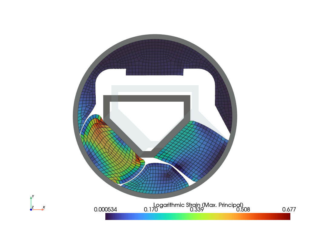
The maximum principal values of the logarithmic strain tensors are plotted on the deformed configuration.

plotter = fields[0].plot(color="grey", show_edges=False)
plotter = fields[1].plot("Principal Values of Logarithmic Strain", plotter=plotter)
plotter.show()

Static Scene

Interactive Scene