Note
Go to the end to download the full example code.
Inflation of a hyperelastic balloon#
This example requires external packages.
pip install contique
With the help of contique it is possible to apply a numerical parameter continuation algorithm on any system of equilibrium equations. This advanced tutorial demonstrates the usage of FElupe in conjunction with contique. The unstable inflation of a circular hyperelastic balloon demonstrates this powerful approach. The deformed model and the pressure - displacement curve is plotted.
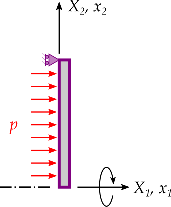
First, setup a problem in FElupe as usual (mesh, region, field, boundaries, umat, solid
and a pressure boundary). For the material definition we use the
Neo-Hooke built-in
hyperelastic material formulation, see Eq. (1).
import contique
import numpy as np

import felupe as fem

mesh = fem.Rectangle(b=(1, 25), n=(2, 4)).add_midpoints_edges().add_midpoints_faces()
region = fem.RegionBiQuadraticQuad(mesh)
field = fem.FieldsMixed(region, n=1, axisymmetric=True)
boundaries = fem.dof.symmetry(field[0], axes=(0, 1))
boundaries["fix-y"] = fem.Boundary(field[0], fy=mesh.y.max(), mode="or", skip=(0, 1))
dof0, dof1 = fem.dof.partition(field, boundaries)

umat = fem.NeoHookeCompressible(mu=1, lmbda=50)
solid = fem.SolidBody(umat, field)

region_for_pressure = fem.RegionBiQuadraticQuadBoundary(
    mesh, mask=(mesh.x == 0), ensure_3d=True
)
field_for_pressure = fem.FieldContainer(
    [fem.FieldAxisymmetric(region_for_pressure, dim=2)]
)

pressure = fem.SolidBodyPressure(field_for_pressure)
The next step involves the problem definition for contique. For details have a look at its README.
def fun(x, lpf, *args):
    "The system vector of equilibrium equations."

    field[0].values.ravel()[dof1] = x
    pressure.update(lpf)

    return fem.tools.fun([solid, pressure], field)[dof1]


def dfundx(x, lpf, *args):
    """The jacobian of the system vector of equilibrium equations w.r.t. the
    primary unknowns."""

    field[0].values.ravel()[dof1] = x
    pressure.update(lpf)

    K = fem.tools.jac(items=[solid, pressure], x=field)

    return fem.solve.partition(field, K, dof1, dof0)[2]


def dfundl(x, lpf, *args):
    """The jacobian of the system vector of equilibrium equations w.r.t. the
    load proportionality factor."""

    pressure.update(1)

    return fem.tools.fun([pressure], field)[dof1]
Next we have to init the problem and specify the initial values of unknowns (the undeformed configuration). After each completed step of the numeric continuation the results are saved.
|Step,C.| Control Component | Norm (Iter.#) | Message     |
|-------|-------------------|---------------|-------------|
|   1,1 |     0+  =>    12+ | 5.8e-07 ( 4#) | => re-Cycle |
|     2 |    12+  =>    12+ | 5.7e-07 ( 4#) |             |
|   2,1 |    12+  =>     0+ | 5.7e-07 ( 4#) | => re-Cycle |
|     2 |     0+  =>     0+ | 5.8e-07 ( 4#) |             |
|   3,1 |     0+  =>     0+ | 9.2e-07 ( 4#) |             |
|   4,1 |     0+  =>     0+ | 2.3e-05 ( 4#) |             |
|   5,1 |     0+  =>     0+ | 5.1e-04 ( 4#) |             |
|   6,1 |     0+  =>     0+ | 4.7e-07 ( 5#) |             |
|   7,1 |     0+  =>     0+ | 1.8e-07 ( 5#) |             |
|   8,1 |     0+  =>     0+ | 8.5e-07 ( 5#) |             |
|   9,1 |     0+  =>     0+ | 1.5e-06 ( 5#) |             |
|  10,1 |     0+  =>    36+ | 2.0e-05 ( 5#) | => re-Cycle |
|     2 |    36+  =>    36+ | 9.1e-05 ( 5#) |             |
|  11,1 |    36+  =>     0+ | 1.9e-07 ( 5#) | => re-Cycle |
|     2 |     0+  =>     0+ | 2.5e-06 ( 7#) |             |
|  12,1 |     0+  =>     0+ | 5.5e-04 ( 5#) |             |
|  13,1 |     0+  =>     0+ | 3.6e-04 ( 4#) |             |
|  14,1 |     0+  =>     0+ | 5.8e-04 ( 4#) |             |
|  15,1 |     0+  =>     0+ | 4.3e-04 ( 4#) |             |
|  16,1 |     0+  =>     0+ | 3.4e-09 ( 5#) |             |
|  17,1 |     0+  =>     0+ | 5.5e-04 ( 4#) |             |
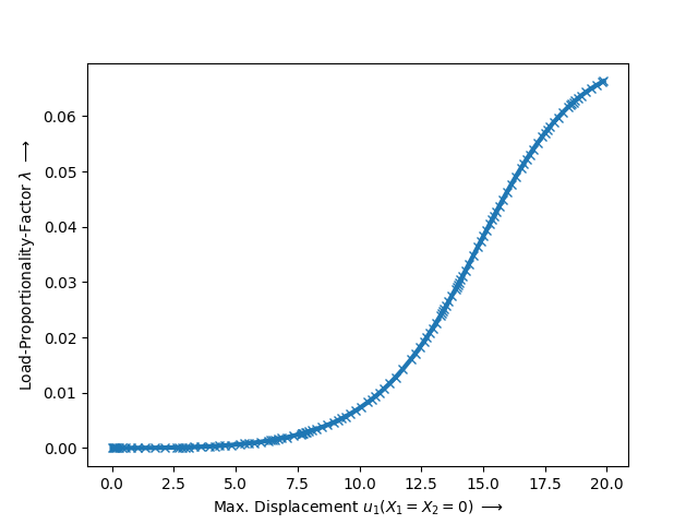
The unstable pressure-controlled equilibrium path is plotted as pressure-displacement curve.
import matplotlib.pyplot as plt

plt.plot(X[:, 0], X[:, -1], "x-", lw=3)
plt.xlabel(r"Max. Displacement $u_1(X_1=X_2=0)$ $\longrightarrow$")
plt.ylabel(r"Load-Proportionality-Factor $\lambda$ $\longrightarrow$")
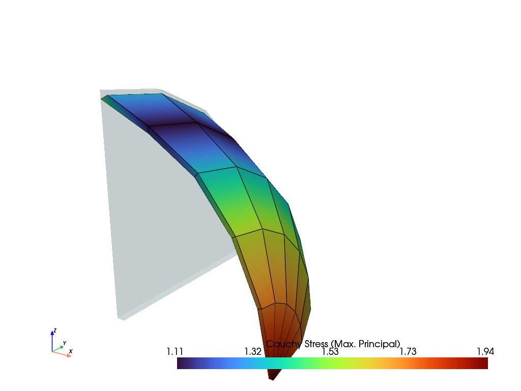
The deformed configuration of the revolved solid body is plotted.
solid.revolve(n=10, phi=90).plot(
    "Principal Values of Cauchy Stress", project=fem.topoints, nonlinear_subdivision=3
).show()
Total running time of the script: (0 minutes 1.613 seconds)