Elastic bearing with torsional loading

An elastic bearing with combined multiaxial loading.

• create and stack meshes

• define a boundary condition with torsional loading

• work with multiple solid bodies

• create a step and add it to a job

• plot strains and stresses

This example requires external packages.

pip install pypardiso

An elastic bearing is subjected to combined multiaxial radial-torsional-cardanic loading. First the meshes for the rubber and the metal sheet rings are created.

import numpy as np
import pypardiso

import felupe as fem

# inner and outer line meshes for the rubber
bottom = fem.mesh.Line(a=-50, b=50, n=6)
top = fem.mesh.Line(a=-30, b=30, n=6)

# embed line meshes in 2d-space
bottom.update(np.pad(bottom.points, ((0, 0), (0, 1)), constant_values=30))
top.update(np.pad(top.points, ((0, 0), (0, 1)), constant_values=60))

# fill face with quads between the two line meshes, add realistic runouts
section = fem.mesh.fill_between(bottom, top, n=8)
section = section.add_runouts(axis=1, centerpoint=[0, 45], values=[0.2], normalize=True)

# revolve the face for the rubber volume
rubber = section.revolve(n=19, phi=360)

# create meshes for the metal sheet rings
metals = [
    fem.Rectangle(a=(-50, 25), b=(50, 30), n=(21, 3)).revolve(n=19, phi=360),
    fem.Rectangle(a=(-30, 60), b=(30, 65), n=(21, 3)).revolve(n=19, phi=360),
]

# stack the meshes
meshes = fem.MeshContainer([rubber, *metals], merge=True)
mesh = fem.mesh.stack(meshes.meshes)
x, y, z = mesh.points.T

mesh.plot().show()

Static Scene

Interactive Scene

A global region as well as sub-regions for all materials are generated. The same applies to the fields, the material formulations as well as the solid bodies.

region = fem.RegionHexahedron(mesh)
regions = [fem.RegionHexahedron(m) for m in meshes]
field = fem.FieldContainer([fem.Field(region, dim=3)])
fields = [fem.FieldContainer([fem.Field(r, dim=3)]) for r in regions]

# material formulations and solid bodies for the rubber and the metal sheets
umats = [fem.NeoHooke(mu=1), fem.LinearElasticLargeStrain(E=2.1e5, nu=0.3)]
solids = [
    fem.SolidBodyNearlyIncompressible(umats[0], fields[0], bulk=5000),
    fem.SolidBody(umats[1], fields[1]),
    fem.SolidBody(umats[1], fields[2]),
]

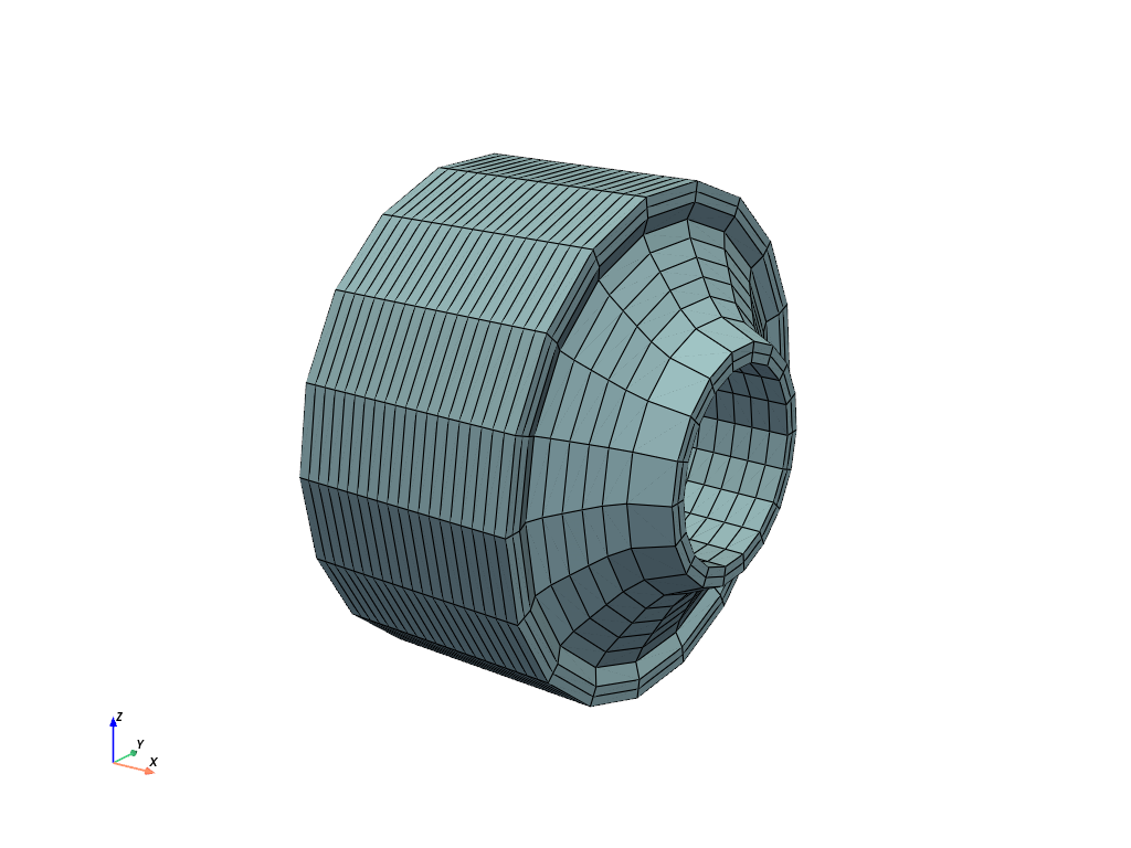
The boundary conditions are created on the global displacement field. Masks are created for both the innermost and the outermost metal sheet faces.

boundaries = {
    "inner": fem.dof.Boundary(field[0], mask=np.isclose(np.sqrt(y**2 + z**2), 25)),
    "outer": fem.dof.Boundary(field[0], mask=np.isclose(np.sqrt(y**2 + z**2), 65)),
}

# prescribed values for the innermost radial mesh points
table = fem.math.linsteps([0, 1], num=3)
move = []

for progress in table:
    inner = mesh.points[boundaries["inner"].points]
    inner_rotated = fem.mesh.rotate(
        points=inner,
        cells=None,
        cell_type=None,
        angle_deg=30 * progress,
        axis=0,
        center=[0, 0, 0],
    )[0]
    inner_rotated = fem.mesh.rotate(
        points=inner_rotated,
        cells=None,
        cell_type=None,
        angle_deg=-5 * progress,
        axis=1,
        center=[0, 0, 0],
    )[0]
    inner_radial = 8 * np.array([0, 0, 1]) * progress
    move.append((inner_radial + inner_rotated - inner).ravel())

After defining the load step, the simulation model is ready to be solved.

step = fem.Step(items=solids, ramp={boundaries["inner"]: move}, boundaries=boundaries)
job = fem.Job(steps=[step])
job.evaluate(x0=field, parallel=True, solver=pypardiso.spsolve)

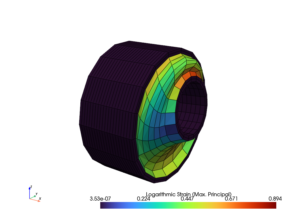
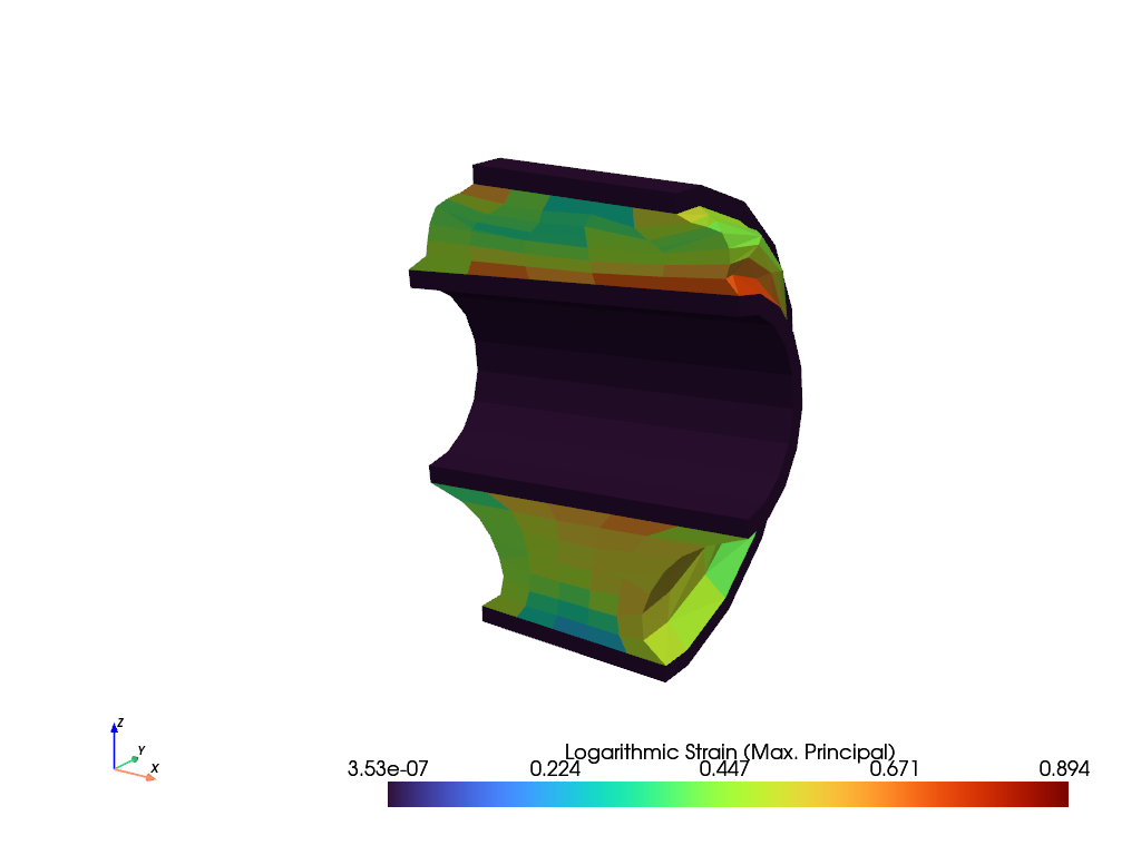
The maximum principal values of the logarithmic strain are plotted on the total simulation model as well as on a clipped view.

field.plot("Principal Values of Logarithmic Strain", show_undeformed=False).show()

plotter = field.plot(
    "Principal Values of Logarithmic Strain",
    show_undeformed=False,
    show_edges=False,
)
plotter.mesh.clip("y", invert=False, value=0.0, inplace=True)
plotter.show()

Static Scene

Interactive Scene

Static Scene

Interactive Scene