Tools & Helpers

This page contains tools and helpers for constitutive material formulations.

View Force-Stretch Curves on Elementary Deformations

ViewMaterial(umat[, ux, ps, bx, statevars])	Create views on normal force per undeformed area vs stretch curves for the elementary homogeneous deformations uniaxial tension/compression, planar shear and biaxial tension of a given isotropic material formulation.
ViewMaterialIncompressible(umat[, ux, ps, ...])	Create views on normal force per undeformed area vs stretch curves for the elementary homogeneous incompressible deformations uniaxial tension/compression, planar shear and biaxial tension of a given isotropic material formulation.

Special Constitutive Materials

CompositeMaterial(material, other_material)	A composite material with two constitutive materials merged.
Volumetric(bulk[, parallel])	Neo-Hookean material formulation with deactivated shear modulus.
LineChange([parallel])	Line Change.
AreaChange([parallel])	Area Change.
VolumeChange([parallel])	Volume Change.

Other

constitution.lame_converter(E, nu)	Convert the pair of given material parameters Young's modulus \(E\) and Poisson ratio \(\nu\) to first and second Lamé - constants \(\lambda\) and \(\mu\).
constitution.lame_converter_orthotropic(E, nu, G)	Convert elastic orthotropic material parameters to Lamé constants.

Detailed API Reference

class felupe.ViewMaterial(umat, ux=array([0.7, 0.75, 0.8, 0.85, 0.9, 0.95, 1., 1.05, 1.1, 1.15, 1.2, 1.25, 1.3, 1.35, 1.4, 1.45, 1.5, 1.55, 1.6, 1.65, 1.7, 1.75, 1.8, 1.85, 1.9, 1.95, 2., 2.05, 2.1, 2.15, 2.2, 2.25, 2.3, 2.35, 2.4, 2.45, 2.5]), ps=array([1., 1.05, 1.1, 1.15, 1.2, 1.25, 1.3, 1.35, 1.4, 1.45, 1.5, 1.55, 1.6, 1.65, 1.7, 1.75, 1.8, 1.85, 1.9, 1.95, 2., 2.05, 2.1, 2.15, 2.2, 2.25, 2.3, 2.35, 2.4, 2.45, 2.5]), bx=array([1., 1.05, 1.1, 1.15, 1.2, 1.25, 1.3, 1.35, 1.4, 1.45, 1.5, 1.55, 1.6, 1.65, 1.7, 1.75]), statevars=None)

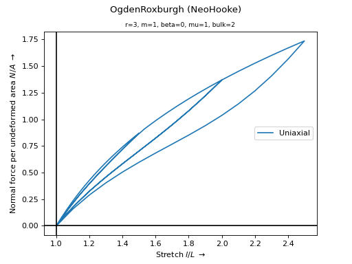
Create views on normal force per undeformed area vs stretch curves for the elementary homogeneous deformations uniaxial tension/compression, planar shear and biaxial tension of a given isotropic material formulation.

Parameters:

• umat (class) – A class with methods for the gradient and hessian of the strain energy density function w.r.t. the deformation gradient. See Material for further details.

• ux (ndarray, optional) – Array with stretches for uniaxial tension/compression. Default is linsteps([0.7, 2.5], num=36).

• ps (ndarray, optional) – Array with stretches for planar shear. Default is linsteps([1.0, 2.5], num=30).

• bx (ndarray, optional) – Array with stretches for equi-biaxial tension. Default is linsteps([1.0, 1.75], num=15)`.

• statevars (ndarray or None, optional) – Array with state variables (default is None). If None, the state variables are assumed to be initially zero.

Examples

>>> import felupe as fem
>>>
>>> umat = fem.OgdenRoxburgh(fem.NeoHooke(mu=1, bulk=2), r=3, m=1, beta=0)
>>> view = fem.ViewMaterial(
...     umat,
...     ux=fem.math.linsteps([1, 1.5, 1, 2, 1, 2.5, 1], num=15),
...     ps=None,
...     bx=None,
... )
>>> ax = view.plot(show_title=True, show_kwargs=True)

biaxial(stretches=None, **kwargs)

Normal force per undeformed area vs stretch curve for a equi-biaxial deformation.

Parameters:

stretches (ndarray or None, optional) – Array with stretches at which the forces are evaluated (default is None). If None, the stretches from initialization are used.

Returns:

3-tuple with array of stretches and array of forces and the label.

Return type:

tuple of ndarray

evaluate()

Evaluate normal force per undeformed area vs stretch curves for the elementary homogeneous incompressible deformations uniaxial tension/compression, planar shear and biaxial tension. A load case is not included if its array of stretches (attribute ux, ps or bx) is None.

Returns:

List with 3-tuple of stretch and force arrays and the label string for each load case.

Return type:

list of 3-tuple

planar(stretches=None, **kwargs)

Normal force per undeformed area vs stretch curve for a planar shear deformation.

Parameters:

stretches (ndarray or None, optional) – Array with stretches at which the forces are evaluated (default is None). If None, the stretches from initialization are used.

Returns:

3-tuple with array of stretches and array of forces and the label.

Return type:

tuple of ndarray

plot(ax=None, show_title=True, show_kwargs=True, **kwargs)

Plot normal force per undeformed area vs stretch curves for the elementary homogeneous incompressible deformations uniaxial tension/compression, planar shear and biaxial tension.

uniaxial(stretches=None, **kwargs)

Normal force per undeformed area vs. stretch curve for a uniaxial deformation.

Parameters:

stretches (ndarray or None, optional) – Array with stretches at which the forces are evaluated (default is None). If None, the stretches from initialization are used.

Returns:

3-tuple with array of stretches and array of forces and the label.

Return type:

tuple of ndarray

class felupe.ViewMaterialIncompressible(umat, ux=array([0.7, 0.75, 0.8, 0.85, 0.9, 0.95, 1., 1.05, 1.1, 1.15, 1.2, 1.25, 1.3, 1.35, 1.4, 1.45, 1.5, 1.55, 1.6, 1.65, 1.7, 1.75, 1.8, 1.85, 1.9, 1.95, 2., 2.05, 2.1, 2.15, 2.2, 2.25, 2.3, 2.35, 2.4, 2.45, 2.5]), ps=array([1., 1.05, 1.1, 1.15, 1.2, 1.25, 1.3, 1.35, 1.4, 1.45, 1.5, 1.55, 1.6, 1.65, 1.7, 1.75, 1.8, 1.85, 1.9, 1.95, 2., 2.05, 2.1, 2.15, 2.2, 2.25, 2.3, 2.35, 2.4, 2.45, 2.5]), bx=array([1., 1.05, 1.1, 1.15, 1.2, 1.25, 1.3, 1.35, 1.4, 1.45, 1.5, 1.55, 1.6, 1.65, 1.7, 1.75]), statevars=None)

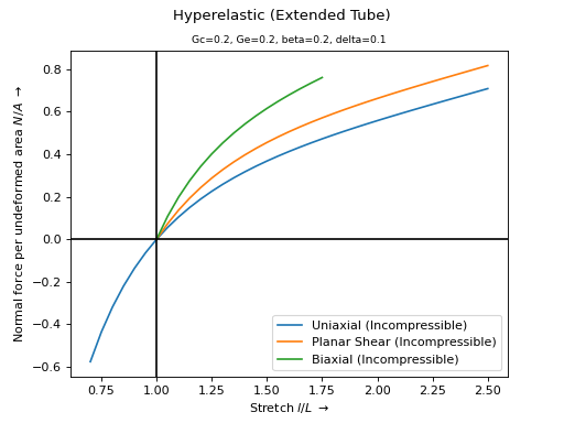
Create views on normal force per undeformed area vs stretch curves for the elementary homogeneous incompressible deformations uniaxial tension/compression, planar shear and biaxial tension of a given isotropic material formulation.

Parameters:

• umat (class) – A class with methods for the gradient and hessian of the strain energy density function w.r.t. the deformation gradient. See Material for further details.

• ux (ndarray, optional) – Array with stretches for incompressible uniaxial tension/compression. Default is linsteps([0.7, 2.5], num=36).

• ps (ndarray, optional) – Array with stretches for incompressible planar shear. Default is linsteps([1, 2.5], num=30).

• bx (ndarray, optional) – Array with stretches for incompressible equi-biaxial tension. Default is linsteps([1, 1.75], num=15).

• statevars (ndarray or None, optional) – Array with state variables (default is None). If None, the state variables are assumed to be initially zero.

Examples

>>> import felupe as fem
>>>
>>> umat = fem.Hyperelastic(fem.extended_tube, Gc=0.2, Ge=0.2, beta=0.2, delta=0.1)
>>> preview = fem.ViewMaterialIncompressible(umat)
>>> ax = preview.plot(show_title=True, show_kwargs=True)

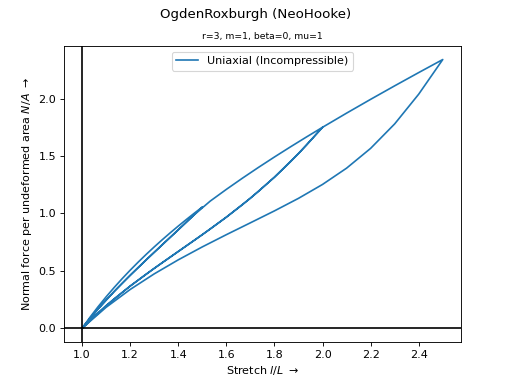
>>> umat = fem.OgdenRoxburgh(fem.NeoHooke(mu=1), r=3, m=1, beta=0)
>>> view = fem.ViewMaterialIncompressible(
...     umat,
...     ux=fem.math.linsteps([1, 1.5, 1, 2, 1, 2.5, 1], num=15),
...     ps=None,
...     bx=None,
... )
>>> ax = view.plot(show_title=True, show_kwargs=True)

biaxial(stretches=None)

Normal force per undeformed area vs stretch curve for a equi-biaxial incompressible deformation.

Parameters:

stretches (ndarray or None, optional) – Array with stretches at which the forces are evaluated (default is None). If None, the stretches from initialization are used.

Returns:

3-tuple with array of stretches and array of forces and the label.

Return type:

tuple of ndarray

evaluate()

Evaluate normal force per undeformed area vs stretch curves for the elementary homogeneous incompressible deformations uniaxial tension/compression, planar shear and biaxial tension. A load case is not included if its array of stretches (attribute ux, ps or bx) is None.

Returns:

List with 3-tuple of stretch and force arrays and the label string for each load case.

Return type:

list of 3-tuple

planar(stretches=None)

Normal force per undeformed area vs stretch curve for a planar shear incompressible deformation.

Parameters:

stretches (ndarray or None, optional) – Array with stretches at which the forces are evaluated (default is None). If None, the stretches from initialization are used.

Returns:

3-tuple with array of stretches and array of forces and the label.

Return type:

tuple of ndarray

plot(ax=None, show_title=True, show_kwargs=True, **kwargs)

Plot normal force per undeformed area vs stretch curves for the elementary homogeneous incompressible deformations uniaxial tension/compression, planar shear and biaxial tension.

uniaxial(stretches=None)

Normal force per undeformed area vs stretch curve for a uniaxial incompressible deformation.

Parameters:

stretches (ndarray or None, optional) – Array with stretches at which the forces are evaluated (default is None). If None, the stretches from initialization are used.

Returns:

3-tuple with array of stretches and array of forces and the label.

Return type:

tuple of ndarray

class felupe.CompositeMaterial(material, other_material)

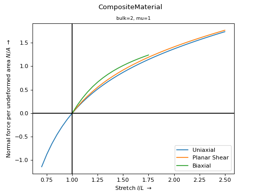
A composite material with two constitutive materials merged. State variables are only considered for the first material.

Parameters:

• material (ConstitutiveMaterial) – First constitutive material.

• other_material (ConstitutiveMaterial) – Second constitutive material.

Notes

Warning

Do not merge two constitutive materials with the same keys of material parameters. In this case, the values of these material parameters are taken from the first constitutive material.

Examples

>>> import felupe as fem
>>>
>>> nh = fem.NeoHooke(mu=1.0)
>>> vol = fem.Volumetric(bulk=2.0)
>>> umat = nh & vol
>>> ax = umat.plot()

copy()

Return a deep-copy of the constitutive material.

gradient(x, **kwargs)

hessian(x, **kwargs)

optimize(ux=None, ps=None, bx=None, incompressible=False, relative=False, **kwargs)

Optimize the material parameters by a least-squares fit on experimental stretch-stress data.

Parameters:

• ux (array of shape (2, ...) or None, optional) – Experimental uniaxial stretch and force-per-undeformed-area data (default is None).

• ps (array of shape (2, ...) or None, optional) – Experimental planar-shear stretch and force-per-undeformed-area data (default is None).

• bx (array of shape (2, ...) or None, optional) – Experimental biaxial stretch and force-per-undeformed-area data (default is None).

• incompressible (bool, optional) – A flag to enforce incompressible deformations (default is False).

• relative (bool, optional) – A flag to optimize relative instead of absolute residuals, i.e. (predicted - observed) / observed instead of predicted - observed (default is False).

• **kwargs (dict, optional) – Optional keyword arguments are passed to scipy.optimize.least_squares().

Returns:

• ConstitutiveMaterial – A copy of the constitutive material with the optimized material parameters.

• scipy.optimize.OptimizeResult – Represents the optimization result.

Notes

Warning

At least one load case, i.e. one of the arguments ux, ps or bx must not be None.

The vector of residuals is given in Eq. (3) in case of absolute residuals

(1)\[ \begin{align}\begin{aligned}\begin{split}\boldsymbol{r} &= \begin{bmatrix} \boldsymbol{r}_\text{ux} \\ \boldsymbol{r}_\text{ps} \\ \boldsymbol{r}_\text{bx} \end{bmatrix}\end{split}\\r_\text{ux}(\lambda_i) &= P_\text{ux}(\lambda_i) - P_\text{ux, observed}(\lambda_i)\\r_\text{ps}(\lambda_i) &= P_\text{ps}(\lambda_i) - P_\text{ps, observed}(\lambda_i)\\r_\text{bx}(\lambda_i) &= P_\text{bx}(\lambda_i) - P_\text{bx, observed}(\lambda_i)\end{aligned}\end{align} \]

and in Eq. (4) in case of relative residuals.

(2)\[ \begin{align}\begin{aligned}\begin{split}\boldsymbol{r} &= \begin{bmatrix} \boldsymbol{r}_\text{ux} \\ \boldsymbol{r}_\text{ps} \\ \boldsymbol{r}_\text{bx} \end{bmatrix}\end{split}\\r_\text{ux}(\lambda_i) &= \frac{ P_\text{ux}(\lambda_i) - P_\text{ux, observed}(\lambda_i)}{ P_\text{ux, observed}(\lambda_i) }\\r_\text{ps}(\lambda_i) &= \frac{ P_\text{ps}(\lambda_i) - P_\text{ps, observed}(\lambda_i)}{ P_\text{ps, observed}(\lambda_i) }\\r_\text{bx}(\lambda_i) &= \frac{ P_\text{bx}(\lambda_i) - P_\text{bx, observed}(\lambda_i)}{ P_\text{bx, observed}(\lambda_i) }\end{aligned}\end{align} \]

Examples

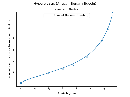
The Anssari-Benam Bucchi material model formulation is best-fitted on Treloar’s uniaxial and biaxial tension data [1]_.

>>> import numpy as np
>>> import felupe as fem
>>>
>>> λ, P = np.array(
...     [
...         [1.000, 0.00],
...         [1.240, 2.30],
...         [1.585, 4.16],
...         [2.180, 6.00],
...         [3.020, 8.80],
...         [4.030, 12.5],
...         [4.760, 16.2],
...         [5.750, 23.6],
...         [6.850, 38.5],
...         [7.250, 49.6],
...         [7.600, 64.4],
...     ]
... ).T * np.array([[1.0], [0.0980665]])
>>>
>>> umat = fem.Hyperelastic(fem.anssari_benam_bucchi)
>>> umat_new, res = umat.optimize(
...     ux=[λ, P], incompressible=True, relative=True
... )
>>>
>>> ux = np.linspace(λ.min(), λ.max(), num=50)
>>> ax = umat_new.plot(incompressible=True, ux=ux, bx=None, ps=None)

>>> ax.plot(λ, P, "C0x")

See also

scipy.optimize.least_squares

Solve a nonlinear least-squares problem with bounds on the variables.

References

[1]

L. R. G. Treloar, “Stress-strain data for vulcanised rubber under various types of deformation”, Transactions of the Faraday Society, vol. 40. Royal Society of Chemistry (RSC), p. 59, 1944. doi: 10.1039/tf9444000059. Data available at https://www.uni-due.de/mathematik/ag_neff/neff_hencky.

plot(incompressible=False, **kwargs)

Return a plot with normal force per undeformed area vs. stretch curves for the elementary homogeneous deformations uniaxial tension/compression, planar shear and biaxial tension of a given isotropic material formulation.

Parameters:

• incompressible (bool, optional) – A flag to enforce views on incompressible deformations (default is False).

• **kwargs (dict, optional) – Optional keyword-arguments for ViewMaterial or ViewMaterialIncompressible.

Return type:

matplotlib.axes.Axes

See also

felupe.ViewMaterial

Create views on normal force per undeformed area vs. stretch curves for the elementary homogeneous deformations uniaxial tension/compression, planar shear and biaxial tension of a given isotropic material formulation.

felupe.ViewMaterialIncompressible

Create views on normal force per undeformed area vs. stretch curves for the elementary homogeneous incompressible deformations uniaxial tension/compression, planar shear and biaxial tension of a given isotropic material formulation.

screenshot(filename='umat.png', incompressible=False, **kwargs)

Save a screenshot with normal force per undeformed area vs. stretch curves for the elementary homogeneous deformations uniaxial tension/compression, planar shear and biaxial tension of a given isotropic material formulation.

Parameters:

• filename (str, optional) – The filename of the screenshot (default is “umat.png”).

• incompressible (bool, optional) – A flag to enforce views on incompressible deformations (default is False).

• **kwargs (dict, optional) – Optional keyword-arguments for ViewMaterial or ViewMaterialIncompressible.

Return type:

matplotlib.axes.Axes

See also

felupe.ViewMaterial

Create views on normal force per undeformed area vs. stretch curves for the elementary homogeneous deformations uniaxial tension/compression, planar shear and biaxial tension of a given isotropic material formulation.

felupe.ViewMaterialIncompressible

Create views on normal force per undeformed area vs. stretch curves for the elementary homogeneous incompressible deformations uniaxial tension/compression, planar shear and biaxial tension of a given isotropic material formulation.

view(incompressible=False, **kwargs)

Create views on normal force per undeformed area vs. stretch curves for the elementary homogeneous deformations uniaxial tension/compression, planar shear and biaxial tension of a given isotropic material formulation.

Parameters:

• incompressible (bool, optional) – A flag to enforce views on incompressible deformations (default is False).

• **kwargs (dict, optional) – Optional keyword-arguments for ViewMaterial or ViewMaterialIncompressible.

Return type:

felupe.ViewMaterial or felupe.ViewMaterialIncompressible

See also

felupe.ViewMaterial

Create views on normal force per undeformed area vs. stretch curves for the elementary homogeneous deformations uniaxial tension/compression, planar shear and biaxial tension of a given isotropic material formulation.

felupe.ViewMaterialIncompressible

Create views on normal force per undeformed area vs. stretch curves for the elementary homogeneous incompressible deformations uniaxial tension/compression, planar shear and biaxial tension of a given isotropic material formulation.

class felupe.Volumetric(bulk, parallel=False)

Neo-Hookean material formulation with deactivated shear modulus.

copy()

Return a deep-copy of the constitutive material.

function(x)

Strain energy density function per unit undeformed volume of the Neo-Hookean material formulation.

Parameters:

x (list of ndarray) – List with the Deformation gradient F (3x3) as first item

gradient(x, out=None)

Gradient of the strain energy density function per unit undeformed volume of the Neo-Hookean material formulation.

Parameters:

• x (list of ndarray) – List with the Deformation gradient F (3x3) as first item

• out (ndarray or None, optional) – A location into which the result is stored (default is None).

hessian(x, out=None)

Hessian of the strain energy density function per unit undeformed volume of the Neo-Hookean material formulation.

Parameters:

• x (list of ndarray) – List with the Deformation gradient F (3x3) as first item

• out (ndarray or None, optional) – A location into which the result is stored (default is None).

optimize(ux=None, ps=None, bx=None, incompressible=False, relative=False, **kwargs)

Optimize the material parameters by a least-squares fit on experimental stretch-stress data.

Parameters:

• ux (array of shape (2, ...) or None, optional) – Experimental uniaxial stretch and force-per-undeformed-area data (default is None).

• ps (array of shape (2, ...) or None, optional) – Experimental planar-shear stretch and force-per-undeformed-area data (default is None).

• bx (array of shape (2, ...) or None, optional) – Experimental biaxial stretch and force-per-undeformed-area data (default is None).

• incompressible (bool, optional) – A flag to enforce incompressible deformations (default is False).

• relative (bool, optional) – A flag to optimize relative instead of absolute residuals, i.e. (predicted - observed) / observed instead of predicted - observed (default is False).

• **kwargs (dict, optional) – Optional keyword arguments are passed to scipy.optimize.least_squares().

Returns:

• ConstitutiveMaterial – A copy of the constitutive material with the optimized material parameters.

• scipy.optimize.OptimizeResult – Represents the optimization result.

Notes

Warning

At least one load case, i.e. one of the arguments ux, ps or bx must not be None.

The vector of residuals is given in Eq. (3) in case of absolute residuals

(3)\[ \begin{align}\begin{aligned}\begin{split}\boldsymbol{r} &= \begin{bmatrix} \boldsymbol{r}_\text{ux} \\ \boldsymbol{r}_\text{ps} \\ \boldsymbol{r}_\text{bx} \end{bmatrix}\end{split}\\r_\text{ux}(\lambda_i) &= P_\text{ux}(\lambda_i) - P_\text{ux, observed}(\lambda_i)\\r_\text{ps}(\lambda_i) &= P_\text{ps}(\lambda_i) - P_\text{ps, observed}(\lambda_i)\\r_\text{bx}(\lambda_i) &= P_\text{bx}(\lambda_i) - P_\text{bx, observed}(\lambda_i)\end{aligned}\end{align} \]

and in Eq. (4) in case of relative residuals.

(4)\[ \begin{align}\begin{aligned}\begin{split}\boldsymbol{r} &= \begin{bmatrix} \boldsymbol{r}_\text{ux} \\ \boldsymbol{r}_\text{ps} \\ \boldsymbol{r}_\text{bx} \end{bmatrix}\end{split}\\r_\text{ux}(\lambda_i) &= \frac{ P_\text{ux}(\lambda_i) - P_\text{ux, observed}(\lambda_i)}{ P_\text{ux, observed}(\lambda_i) }\\r_\text{ps}(\lambda_i) &= \frac{ P_\text{ps}(\lambda_i) - P_\text{ps, observed}(\lambda_i)}{ P_\text{ps, observed}(\lambda_i) }\\r_\text{bx}(\lambda_i) &= \frac{ P_\text{bx}(\lambda_i) - P_\text{bx, observed}(\lambda_i)}{ P_\text{bx, observed}(\lambda_i) }\end{aligned}\end{align} \]

Examples

The Anssari-Benam Bucchi material model formulation is best-fitted on Treloar’s uniaxial and biaxial tension data [1]_.

>>> import numpy as np
>>> import felupe as fem
>>>
>>> λ, P = np.array(
...     [
...         [1.000, 0.00],
...         [1.240, 2.30],
...         [1.585, 4.16],
...         [2.180, 6.00],
...         [3.020, 8.80],
...         [4.030, 12.5],
...         [4.760, 16.2],
...         [5.750, 23.6],
...         [6.850, 38.5],
...         [7.250, 49.6],
...         [7.600, 64.4],
...     ]
... ).T * np.array([[1.0], [0.0980665]])
>>>
>>> umat = fem.Hyperelastic(fem.anssari_benam_bucchi)
>>> umat_new, res = umat.optimize(
...     ux=[λ, P], incompressible=True, relative=True
... )
>>>
>>> ux = np.linspace(λ.min(), λ.max(), num=50)
>>> ax = umat_new.plot(incompressible=True, ux=ux, bx=None, ps=None)

>>> ax.plot(λ, P, "C0x")

See also

scipy.optimize.least_squares

Solve a nonlinear least-squares problem with bounds on the variables.

References

[1]

L. R. G. Treloar, “Stress-strain data for vulcanised rubber under various types of deformation”, Transactions of the Faraday Society, vol. 40. Royal Society of Chemistry (RSC), p. 59, 1944. doi: 10.1039/tf9444000059. Data available at https://www.uni-due.de/mathematik/ag_neff/neff_hencky.

plot(incompressible=False, **kwargs)

Return a plot with normal force per undeformed area vs. stretch curves for the elementary homogeneous deformations uniaxial tension/compression, planar shear and biaxial tension of a given isotropic material formulation.

Parameters:

• incompressible (bool, optional) – A flag to enforce views on incompressible deformations (default is False).

• **kwargs (dict, optional) – Optional keyword-arguments for ViewMaterial or ViewMaterialIncompressible.

Return type:

matplotlib.axes.Axes

See also

felupe.ViewMaterial

Create views on normal force per undeformed area vs. stretch curves for the elementary homogeneous deformations uniaxial tension/compression, planar shear and biaxial tension of a given isotropic material formulation.

felupe.ViewMaterialIncompressible

Create views on normal force per undeformed area vs. stretch curves for the elementary homogeneous incompressible deformations uniaxial tension/compression, planar shear and biaxial tension of a given isotropic material formulation.

screenshot(filename='umat.png', incompressible=False, **kwargs)

Save a screenshot with normal force per undeformed area vs. stretch curves for the elementary homogeneous deformations uniaxial tension/compression, planar shear and biaxial tension of a given isotropic material formulation.

Parameters:

• filename (str, optional) – The filename of the screenshot (default is “umat.png”).

• incompressible (bool, optional) – A flag to enforce views on incompressible deformations (default is False).

• **kwargs (dict, optional) – Optional keyword-arguments for ViewMaterial or ViewMaterialIncompressible.

Return type:

matplotlib.axes.Axes

See also

felupe.ViewMaterial

Create views on normal force per undeformed area vs. stretch curves for the elementary homogeneous deformations uniaxial tension/compression, planar shear and biaxial tension of a given isotropic material formulation.

felupe.ViewMaterialIncompressible

Create views on normal force per undeformed area vs. stretch curves for the elementary homogeneous incompressible deformations uniaxial tension/compression, planar shear and biaxial tension of a given isotropic material formulation.

view(incompressible=False, **kwargs)

Create views on normal force per undeformed area vs. stretch curves for the elementary homogeneous deformations uniaxial tension/compression, planar shear and biaxial tension of a given isotropic material formulation.

Parameters:

• incompressible (bool, optional) – A flag to enforce views on incompressible deformations (default is False).

• **kwargs (dict, optional) – Optional keyword-arguments for ViewMaterial or ViewMaterialIncompressible.

Return type:

felupe.ViewMaterial or felupe.ViewMaterialIncompressible

See also

felupe.ViewMaterial

Create views on normal force per undeformed area vs. stretch curves for the elementary homogeneous deformations uniaxial tension/compression, planar shear and biaxial tension of a given isotropic material formulation.

felupe.ViewMaterialIncompressible

Create views on normal force per undeformed area vs. stretch curves for the elementary homogeneous incompressible deformations uniaxial tension/compression, planar shear and biaxial tension of a given isotropic material formulation.

class felupe.LineChange(parallel=False)

Line Change.

\[d\boldsymbol{x} = \boldsymbol{F} d\boldsymbol{X}\]

Gradient:

\[\frac{\partial \boldsymbol{F}}{\partial \boldsymbol{F}} = \boldsymbol{I} \overset{ik}{\otimes} \boldsymbol{I}\]

function(extract)

Line change.

Parameters:

extract (list of ndarray) – List of extracted field values with Deformation gradient as first item.

Returns:

F – Deformation gradient

Return type:

ndarray

gradient(extract, parallel=None)

Gradient of line change.

Parameters:

extract (list of ndarray) – List of extracted field values with Deformation gradient as first item.

Returns:

Gradient of line change

Return type:

ndarray

class felupe.AreaChange(parallel=False)

Area Change.

\[d\boldsymbol{a} = J \boldsymbol{F}^{-T} d\boldsymbol{A}\]

Gradient:

\[\frac{\partial J \boldsymbol{F}^{-T}}{\partial \boldsymbol{F}} = J \left( \boldsymbol{F}^{-T} \otimes \boldsymbol{F}^{-T} - \boldsymbol{F}^{-T} \overset{il}{\otimes} \boldsymbol{F}^{-T} \right)\]

function(extract, N=None, parallel=None)

Area change.

Parameters:

• extract (list of ndarray) – List of extracted field values with Deformation gradient as first item.

• N (ndarray or None, optional) – Area normal vector (default is None)

Returns:

Cofactor matrix of the deformation gradient

Return type:

ndarray

gradient(extract, N=None, parallel=None)

Gradient of area change.

Parameters:

• extract (list of ndarray) – List of extracted field values with Deformation gradient as first item.

• N (ndarray or None, optional) – Area normal vector (default is None)

Returns:

Gradient of cofactor matrix of the deformation gradient

Return type:

ndarray

class felupe.VolumeChange(parallel=False)

Volume Change.

\[d\boldsymbol{v} = \text{det}(\boldsymbol{F}) d\boldsymbol{V}\]

Gradient and hessian (equivalent to gradient of area change):

\[ \begin{align}\begin{aligned}\frac{\partial J}{\partial \boldsymbol{F}} &= J \boldsymbol{F}^{-T}\\\frac{\partial^2 J}{\partial \boldsymbol{F}\ \partial \boldsymbol{F}} &= J \left( \boldsymbol{F}^{-T} \otimes \boldsymbol{F}^{-T} - \boldsymbol{F}^{-T} \overset{il}{\otimes} \boldsymbol{F}^{-T} \right)\end{aligned}\end{align} \]

function(extract)

Gradient of volume change.

Parameters:

extract (list of ndarray) – List of extracted field values with Deformation gradient as first item.

Returns:

J – Determinant of the deformation gradient

Return type:

ndarray

gradient(extract)

Gradient of volume change.

Parameters:

F (ndarray) – Deformation gradient

Returns:

Gradient of the determinant of the deformation gradient

Return type:

ndarray

hessian(extract, parallel=None)

Hessian of volume change.

Parameters:

extract (list of ndarray) – List of extracted field values with Deformation gradient as first item.

Returns:

Hessian of the determinant of the deformation gradient

Return type:

ndarray

felupe.constitution.lame_converter(E, nu)

Convert the pair of given material parameters Young’s modulus \(E\) and Poisson ratio \(\nu\) to first and second Lamé - constants \(\lambda\) and \(\mu\).

Parameters:

• E (float) – Young’s modulus.

• nu (float) – Poisson ratio.

Returns:

• lmbda (float) – First Lamé - constant.

• mu (float) – Second Lamé - constant (shear modulus).

Notes

\[ \begin{align}\begin{aligned}\lambda &= \frac{E \nu}{(1 + \nu) (1 - 2 \nu)}\\\mu &= \frac{E}{2 (1 + \nu)}\end{aligned}\end{align} \]

felupe.constitution.lame_converter_orthotropic(E, nu, G)

Convert elastic orthotropic material parameters to Lamé constants.

Parameters:

• E (list of float) – List of the three elastic moduli \(E_1, E_2, E_3\).

• nu (list of float) – List of three poisson ratios \(\nu_{12}, \nu_{23}, \nu_{31}\).

• G (list of float) – List of three shear moduli \(G_{12}, G_{23}, G_{31}\).

Returns:

• lmbda (list of float) – List of six (upper triangle) first Lamé parameters \(\lambda_{11}, \lambda_{12}, \lambda_{13}, \lambda_{22}, \lambda_{23}, \lambda_{33}\).

• mu (list of float) – List of the three second Lamé parameters \(\mu_1,\mu_2, \mu_3\).

Notes

The orthotropic material parameters are converted to orthotropic Lamé constants.

The compliance matrix as the inverse of the stiffness matrix with the parameters \(E_i\), \(\nu_{ij}\) and \(G_{ij}\) is given in Eq. (6).

(5)\[\begin{split}\boldsymbol{C}^{-1} = \begin{bmatrix} \frac{1}{E_1} & -\frac{\nu_{21}}{E_2} & -\frac{\nu_{31}}{E_3} & 0 & 0 & 0 \\ -\frac{\nu_{12}}{E_1} & \frac{1}{E_2} & -\frac{\nu_{32}}{E_3} & 0 & 0 & 0 \\ -\frac{\nu_{13}}{E_1} & -\frac{\nu_{23}}{E_2} & \frac{1}{E_3} & 0 & 0 & 0 \\ 0 & 0 & 0 & \frac{1}{G_{12}} & 0 & 0 \\ 0 & 0 & 0 & 0 & \frac{1}{G_{23}} & 0 \\ 0 & 0 & 0 & 0 & 0 & \frac{1}{G_{31}} \end{bmatrix}\end{split}\]

The stiffness matrix with the Lamé constants is denoted in Eq. ortho-matrix.

(6)\[\begin{split}\boldsymbol{C} = \begin{bmatrix} \lambda_{11} + 2 \mu_1 & \lambda_{12} & \lambda_{13} & 0 & 0 & 0 \\ \lambda_{11} & \lambda_{12} + 2 \mu_2 & \lambda_{13} & 0 & 0 & 0 \\ \lambda_{11} & \lambda_{12} & \lambda_{13} + 2 \mu_3 & 0 & 0 & 0 \\ 0 & 0 & 0 & \frac{\mu_1 + \mu_2}{2} & 0 & 0 \\ 0 & 0 & 0 & 0 & \frac{\mu_2 + \mu_3}{2} & 0 \\ 0 & 0 & 0 & 0 & 0 & \frac{\mu_3 + \mu_1}{2} \end{bmatrix}\end{split}\]

Eq. (6) is evaluated and inverted numerically to extract the Lamé constants.

See also

felupe.LinearElasticOrthotropic

Orthotropic linear-elastic material formulation.

felupe.constitution.tensortrax.models.hyperelastic.saint_venant_kirchhoff_orthotropic

Strain energy function of the orthotropic hyperelastic Saint-Venant Kirchhoff material formulation.